32. Incorrect Models#
GPU
This lecture was built using a machine with access to a GPU — although it will also run without one.
Google Colab has a free tier with GPUs that you can access as follows:
Click on the “play” icon top right
Select Colab
Set the runtime environment to include a GPU
!pip install numpyro
32.1. Overview#
This is a sequel to Likelihood Ratio Processes and Bayesian Learning.
We discuss two ways to create a compound lottery and their consequences.
A compound lottery can be said to create a mixture distribution.
Our two ways of constructing a compound lottery will differ in their timing.
in one, mixing between two possible probability distributions will occur once and for all at the beginning of time
in the other, mixing between the same two possible probability distributions will occur each period
The statistical setting is close but not identical to the problem studied in that lecture.
In that lecture, there were two IID processes that could possibly govern successive draws of a non-negative random variable \(W\).
Nature decided once and for all whether to make a sequence of IID draws from either \( f \) or from \( g \).
That lecture studied an agent who knew both \(f\) and \(g\) but did not know which distribution nature chose at time \(-1\).
The agent represented that ignorance by assuming that nature had chosen \(f\) or \(g\) by flipping an unfair coin that put probability \(\pi_{-1}\) on probability distribution \(f\).
That assumption allowed the agent to construct a subjective joint probability distribution over the random sequence \(\{W_t\}_{t=0}^\infty\).
We studied how the agent would then use the laws of conditional probability and an observed history \(w^t =\{w_s\}_{s=0}^t\) to form
where \(q \in \{f, g\}\) denotes the distribution that nature chose.
However, in the setting of this lecture, that rule imputes to the agent an incorrect model.
The reason is that now the wage sequence is actually described by a different statistical model.
Thus, we change the specification in Likelihood Ratio Processes and Bayesian Learning in the following way.
Now, each period \(t \geq 0\), nature flips a possibly unfair coin that comes up \(f\) with probability \(\alpha\) and \(g\) with probability \(1 -\alpha\).
Thus, nature perpetually draws from the mixture distribution with CDF
and density
We’ll study two agents who try to learn about the wage process, but who use different statistical models.
Both types of agent know \(f\) and \(g\) but neither knows \(\alpha\).
Our first type of agent erroneously thinks that at time \(-1\), nature once and for all chose \(f\) or \(g\) and thereafter permanently draws from that distribution.
Our second type of agent knows, correctly, that nature mixes \(f\) and \(g\) with mixing probability \(\alpha \in (0,1)\) each period, though the agent doesn’t know the mixing parameter.
Our first type of agent applies the learning algorithm described in Likelihood Ratio Processes and Bayesian Learning.
In the context of the statistical model that prevailed in that lecture, that was a good learning algorithm and it enabled the Bayesian learner eventually to learn the distribution that nature had drawn at time \(-1\).
This is because the agent’s statistical model was correct in the sense of being aligned with the data generating process.
But in the present context, our type 1 decision maker’s model is incorrect because the model \(h\) that actually generates the data is neither \(f\) nor \(g\) and so is beyond the support of the models that the agent thinks are possible.
Nevertheless, we’ll see that our first type of agent muddles through and eventually learns something interesting and useful, even though it is not true.
Instead, it turns out that our type 1 agent who is armed with a wrong statistical model ends up learning whichever probability distribution, \(f\) or \(g\), is in a special sense closest to the \(h\) that actually generates the data.
We’ll tell the sense in which it is closest.
Our second type of agent understands that nature mixes between \(f\) and \(g\) each period with a fixed mixing probability \(\alpha\).
But the agent doesn’t know \(\alpha\).
The agent sets out to learn \(\alpha\) using Bayes’ law applied to his model.
His model is correct in the sense that it includes the actual data generating process \(h\) as a possible distribution.
Both agents’ statistical models are exchangeable mixtures of IID sequences of the kind described by de Finetti’s theorem in Exchangeability and Bayesian Updating.
The type 1 agent’s mixing measure puts probability \(\pi_{-1}\) on IID draws from \(f\) and probability \(1 - \pi_{-1}\) on IID draws from \(g\).
The type 2 agent’s mixing measure is a prior density \(\pi_{-1}(\alpha)\) over IID draws from \(h(\cdot|\alpha)\), \(\alpha \in (0,1)\).
Nature’s process, IID draws from \(h(\cdot|\alpha)\), lies inside the support of the type 2 agent’s mixing measure and outside the support of the type 1 agent’s mixing measure.
That is the sense in which the type 1 agent’s model is misspecified.
The two timings of mixing leave different marks on the data.
When nature mixes anew each period, successive draws are independent and \(\textrm{Cov}(W_0, W_1) = 0\).
When nature mixes once and for all with probability \(\pi\) on \(f\), \(\textrm{Cov}(W_0, W_1) = \pi(1-\pi)(\mu_f - \mu_g)^2\), where \(\mu_f\) and \(\mu_g\) are the means of \(f\) and \(g\); see Exercise Exercise 28.1 in Exchangeability and Bayesian Updating.
Merging of Opinions: The Blackwell–Dubins Theorem studies agents who, like our type 2 agent, mix IID sequences with a prior over a parameter.
In this lecture, we’ll learn about
how nature can mix between two distributions \(f\) and \(g\) to create a new distribution \(h\).
The Kullback-Leibler statistical divergence that governs statistical learning under an incorrect statistical model
A useful Python function
numpy.searchsortedthat, in conjunction with a uniform random number generator, can be used to sample from an arbitrary distribution
As usual, we’ll start by importing some Python tools.
import matplotlib.pyplot as plt
import seaborn as sns
import numpy as np
from scipy.integrate import quad
from scipy.optimize import brentq, minimize_scalar
from scipy.special import expit, logit

import numpyro
import jax
import numpyro.distributions as dist
from numpyro.infer import MCMC, NUTS
import jax.numpy as jnp
import jax.scipy.stats as jsp
from jax import random
from jax.scipy.special import gamma

# Enable JAX to use 64-bit float operations
jax.config.update("jax_enable_x64", True)

colors = sns.color_palette()
Let’s use Python to generate two Beta distributions.
# Parameters in the two beta distributions.
F_a, F_b = 1, 1
G_a, G_b = 3, 1.2


@jax.jit
def p(x, a, b):
    r = gamma(a + b) / (gamma(a) * gamma(b))
    return r * x**(a-1) * (1 - x)**(b-1)

# The two density functions.
f = jax.jit(lambda x: p(x, F_a, F_b))
g = jax.jit(lambda x: p(x, G_a, G_b))
32.2. Sampling from compound lottery \(H\)#
We implement two methods to draw samples from our mixture model \(\alpha F + (1-\alpha) G\).
We’ll generate samples using each of them and verify that they match well.
Here is pseudo code for a direct “method 1” for drawing from our compound lottery:
Step one:
use a uniform random draw to flip an unfair coin that selects distribution \(F\) with prob \(\alpha\) and \(G\) with prob \(1 -\alpha\)
Step two:
draw from either \(F\) or \(G\), as determined by the coin flip.
Step three:
put the first two steps in a big loop and do them for each realization of \(w\)
Our second method uses a uniform distribution and the following fact that we also described and used in Some Probability Distributions:
If a random variable \(X\) has CDF \(F\), then a random variable \(F^{-1}(U)\) also has CDF \(F\), where \(U\) is a uniform random variable on \([0,1]\).
In other words, if \(X \sim F(x)\) we can generate a random sample from \(F\) by drawing a random sample from a uniform distribution on \([0,1]\) and computing \(F^{-1}(U)\).
We’ll use this fact
in conjunction with the numpy.searchsorted command to sample from \(H\) directly.
See the numpy.searchsorted documentation for details on the searchsorted function.
In the Python code below, we’ll use both of our methods and confirm that each of them does a good job of sampling from our target mixture distribution.
def draw_lottery(key, α, N):
    """Draw from the compound lottery directly."""
    # split the key: one for the coin flip, one for each distribution
    key_uniform, key_beta1, key_beta2 = jax.random.split(key, 3)

    u = jax.random.uniform(key_uniform, shape=(N,))
    f_draws = jax.random.beta(key_beta1, F_a, F_b, shape=(N,))
    g_draws = jax.random.beta(key_beta2, G_a, G_b, shape=(N,))

    # select F with probability α, else G
    return jnp.where(u <= α, f_draws, g_draws)


# JIT-compile with `N` as a static argument
draw_lottery = jax.jit(draw_lottery, static_argnums=(2,))
def draw_lottery_MC(key, α, N):
    "Draw from the compound lottery using the Monte Carlo trick."

    xs = jnp.linspace(1e-8, 1 - (1e-8), 10000)
    CDF = α * jsp.beta.cdf(xs, F_a, F_b) + (1 - α) * jsp.beta.cdf(xs, G_a, G_b)

    Us = jax.random.uniform(key, shape=(N,))
    draws = xs[jnp.searchsorted(CDF[:-1], Us)]
    return draws
# verify
N = 100000
α = 0.6

key1, key2 = jax.random.split(jax.random.key(42))
sample1 = draw_lottery(key1, α, N)
sample2 = draw_lottery_MC(key2, α, N)

# plot draws and density function
plt.hist(sample1, 50, density=True, alpha=0.5, label="direct draws")
plt.hist(sample2, 50, density=True, alpha=0.5, label="MC draws")

xs = np.linspace(0, 1, 1000)
plt.plot(xs, α * f(xs) + (1 - α) * g(xs), color="red", label="density", lw=2)

plt.legend()
plt.show()
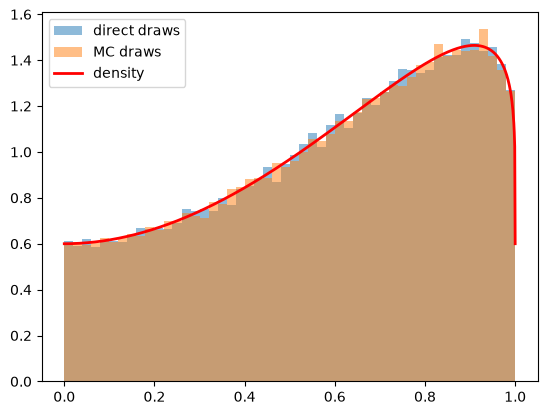
Fig. 32.1 Direct and Monte Carlo draws#
32.3. Type 1 agent#
We’ll now study what our type 1 agent learns.
Remember that our type 1 agent uses the wrong statistical model, thinking that nature mixed between \(f\) and \(g\) once and for all at time \(-1\).
The type 1 agent thus uses the learning algorithm studied in Likelihood Ratio Processes and Bayesian Learning.
We’ll briefly review that learning algorithm now.
Let \( \pi_t \) be a Bayesian posterior defined as
The likelihood ratio process plays a principal role in the formula that governs the evolution of the posterior probability \( \pi_t \), an instance of Bayes’ law.
Bayes’ law implies that \( \{\pi_t\} \) obeys the recursion
with \( \pi_{-1} \) being a Bayesian prior probability that \( q = f \), i.e., a personal or subjective belief about \( q \) based on our having seen no data.
Here \(\ell(w) = f(w)/g(w)\) is the likelihood ratio.
Iterating on (32.1), as in Likelihood Ratio Processes and Bayesian Learning, expresses the time \(t\) posterior \(\pi_t\) as a function of the prior \(\pi_{-1}\) and the likelihood ratio process \(L(w^t) = \prod_{s=0}^{t} \ell(w_s)\):
Formula (32.2) can be regarded as a one step revision of prior probability \( \pi_{-1} \) after seeing the batch of data \( \left\{ w_{s}\right\} _{s=0}^{t} \).
In terms of log odds, formula (32.2) is
Our code computes \(\pi_t\) from (32.3).
Iterating on (32.1) in floating point arithmetic accumulates rounding errors once \(\pi_t\) gets close to \(0\) or \(1\).
32.4. What a type 1 agent learns when mixture \(H\) generates data#
We now study what happens when the mixture distribution \(h(\cdot|\alpha)\) truly generated the data each period.
For all but one value of \(\alpha\), the sequence \(\pi_t\) continues to converge, despite the agent’s misspecified model, and the limit is either \(0\) or \(1\).
This is true even though in truth nature always mixes between \(f\) and \(g\).
After verifying that claim about possible limit points of \(\pi_t\) sequences, we’ll drill down and study what fundamental force determines the limiting value of \(\pi_t\).
Let’s set a value of \(\alpha\) and then watch how \(\pi_t\) evolves.
def simulate_mixed(key, α, T=50, N=500):
    """
    Generate N sets of T observations of the likelihood ratio,
    return as N x T matrix, when the true density is h(·|α)
    """

    w_s = draw_lottery(key, α, N * T).reshape(N, T)
    l_arr = f(w_s) / g(w_s)
    return l_arr


def plot_π_seq(key, α, π1=0.2, π2=0.8, T=200):
    """
    Compute and plot π_t for two priors and the log likelihood ratio process
    when the mixture h(·|α) governs the data.
    """

    l_arr_mixed = simulate_mixed(key, α, T=T, N=1)
    log_L = np.cumsum(np.log(l_arr_mixed[0]))    # log L(w^t), t = 0, ..., T-1

    # plot
    fig, ax1 = plt.subplots()
    for π_init in (π1, π2):
        π_path = expit(logit(π_init) + log_L)
        ax1.plot(
            range(-1, T),
            np.concatenate(([π_init], π_path)),
            label=rf"$\pi_{{-1}}$={π_init}",
            lw=2,
        )

    ax1.plot(
        np.nan, np.nan, "--", color="b",
        label="Log likelihood ratio process", lw=2,
    )
    ax1.set_ylabel(r"$\pi_t$")
    ax1.set_xlabel("$t$")
    ax1.legend()

    ax2 = ax1.twinx()
    ax2.plot(range(T), log_L, "--", color="b", lw=2)
    ax2.set_ylabel(r"$\log(L(w^{t}))$")

    plt.show()
plot_π_seq(jax.random.key(42), α=0.6)
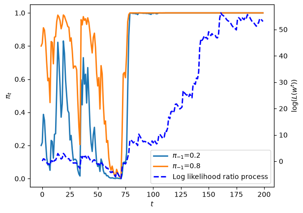
Fig. 32.2 Belief paths, \(\alpha = 0.6\)#
The above graph shows a sample path of the log likelihood ratio process as the blue dashed line, together with sample paths of \(\pi_t\) that start from two distinct initial conditions.
Let’s see what happens when we change \(\alpha\).
plot_π_seq(jax.random.key(42), α=0.2)
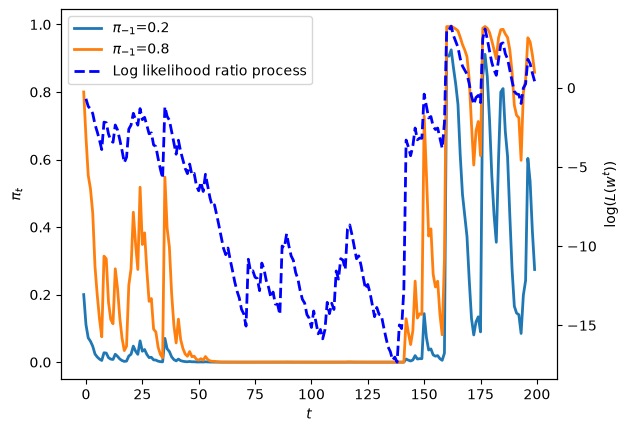
Fig. 32.3 Belief paths, \(\alpha = 0.2\)#
Evidently, \(\alpha\) is having a big effect on the destination of \(\pi_t\) as \(t \rightarrow +\infty\).
32.5. Kullback-Leibler divergence governs limit of \(\pi_t\)#
To understand what determines whether the limit point of \(\pi_t\) is \(0\) or \(1\) and how the answer depends on the true value of the mixing probability \(\alpha \in (0,1)\) that generates
we shall compute the following two Kullback-Leibler divergences
and
We shall plot both of these functions against \(\alpha\) as we use \(\alpha\) to vary \(h(w|\alpha)\).
Because \(\log \ell(w) = \log \frac{h(w|\alpha)}{g(w)} - \log \frac{h(w|\alpha)}{f(w)}\),
where \(E_h\) denotes the expectation under \(h(\cdot|\alpha)\); see A helpful formula and A third distribution h in Likelihood Ratio Processes.
By the law of large numbers, \(\frac{1}{t+1} \log L(w^t)\) converges to \(KL_g(\alpha) - KL_f(\alpha)\) with probability one.
Formula (32.3) then implies that the limit of \(\pi_t\) is determined by
As \(t \rightarrow +\infty\), \(\pi_t\) goes to one if \(KL_f(\alpha) < KL_g(\alpha)\) and goes to zero if \(KL_f(\alpha) > KL_g(\alpha)\).
@jax.jit
def KL_g(α):
    "Compute the KL divergence KL(h, g)."
    err = 1e-8  # to avoid 0 at end points
    ws = jnp.linspace(err, 1 - err, 10000)
    gs, fs = g(ws), f(ws)
    hs = α * fs + (1 - α) * gs
    return jnp.sum(jnp.log(hs / gs) * hs) / 10000


KL_g_v = jax.vmap(KL_g)


@jax.jit
def KL_f(α):
    "Compute the KL divergence KL(h, f)."
    err = 1e-8  # to avoid 0 at end points
    ws = jnp.linspace(err, 1 - err, 10000)
    gs, fs = g(ws), f(ws)
    hs = α * fs + (1 - α) * gs
    return jnp.sum(jnp.log(hs / fs) * hs) / 10000


KL_f_v = jax.vmap(KL_f)


@jax.jit
def π_lim(key, α, T=5000, π_init=0.4):
    """Compute π_{T-1} from the log odds formula eq:logodds_mix."""
    # Get lottery draws
    l_arr = simulate_mixed(key, α, T, N=1)[0]
    log_odds = jnp.log(π_init / (1 - π_init)) + jnp.sum(jnp.log(l_arr))
    return jax.nn.sigmoid(log_odds)


π_lim_v = jax.vmap(π_lim)
Let us first plot the KL divergences \(KL_g\left(\alpha\right), KL_f\left(\alpha\right)\) for each \(\alpha\).
α_arr = np.linspace(0, 1, 100)
KL_g_arr = KL_g_v(α_arr)
KL_f_arr = KL_f_v(α_arr)

fig, ax = plt.subplots()

ax.plot(α_arr, KL_g_arr, label="KL(h, g)", lw=2)
ax.plot(α_arr, KL_f_arr, label="KL(h, f)", lw=2)
ax.set_ylabel("KL divergence")
ax.set_xlabel(r"$\alpha$")

ax.legend(loc="upper right")
plt.show()
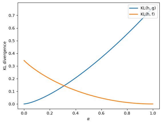
Fig. 32.4 KL divergences against \(\alpha\)#
Let’s compute the \(\alpha^*\) at which the KL divergence between \(h\) and \(g\) equals that between \(h\) and \(f\).
Because \(E_h[\log \ell(w)] = \alpha E_f[\log \ell(w)] + (1-\alpha) E_g[\log \ell(w)] = \alpha KL(f, g) - (1-\alpha) KL(g, f)\), the difference \(KL_g(\alpha) - KL_f(\alpha)\) is linear in \(\alpha\) and
def KL(q1, q2):
    "KL(q1, q2) computed with scipy's quad."
    return quad(lambda w: q1(w) * np.log(q1(w) / q2(w)), 0, 1)[0]

KL_fg, KL_gf = KL(f, g), KL(g, f)
α_star = KL_gf / (KL_fg + KL_gf)

h_star = lambda w: α_star * f(w) + (1 - α_star) * g(w)
print(f"α* = {α_star:.4f}")
print(f"KL(h, f) = {KL(h_star, f):.4f}, KL(h, g) = {KL(h_star, g):.4f} at α*")
α* = 0.3116
KL(h, f) = 0.1435, KL(h, g) = 0.1435 at α*
At \(\alpha^*\), \(f\) and \(g\) both minimize \(KL(h, q)\) over \(q \in \{f, g\}\).
There \(\log L(w^t)\) is a random walk whose increments have mean zero.
Such a random walk is recurrent: with probability one it takes arbitrarily large positive and arbitrarily large negative values infinitely often.
So when \(\alpha = \alpha^*\), \(\pi_t\) does not converge; it keeps returning to values near \(0\) and values near \(1\).
Exercise Exercise 32.2 studies this case.
We can compute and plot \(\pi_{T-1}\) with \(T = 5000\) for each \(\alpha\) on our grid to verify that the convergence is governed by the KL divergence.
The blue circles show the values of \(\pi_{T-1}\) that simulations discover for different values of \(\alpha\) recorded on the \(x\) axis.
The dotted vertical line marks \(\alpha^*\).
keys = jax.random.split(jax.random.key(42), len(α_arr))
π_lim_arr = π_lim_v(keys, α_arr)

# plot
fig, ax = plt.subplots()

ax.plot(α_arr, KL_g_arr, label="KL(h, g)", lw=2)
ax.plot(α_arr, KL_f_arr, label="KL(h, f)", lw=2)
ax.axvline(α_star, color="k", linestyle=":", lw=1)
ax.set_ylabel("KL divergence")
ax.set_xlabel(r"$\alpha$")

# plot KL
ax2 = ax.twinx()
# plot limit point
ax2.scatter(
    α_arr,
    π_lim_arr,
    facecolors="none",
    edgecolors="tab:blue",
    label=r"$\pi_{T-1}$",
)
ax2.set_ylabel(r"$\pi_{T-1}$")

ax.legend(loc=[0.85, 0.8])
ax2.legend(loc=[0.85, 0.73])
plt.show()

wrong_side = (((α_arr < α_star) & (π_lim_arr > 0.5))
              | ((α_arr > α_star) & (π_lim_arr < 0.5)))
print("values of α at which π_{T-1} lies on the side opposite to its limit:",
      np.round(α_arr[wrong_side], 3))
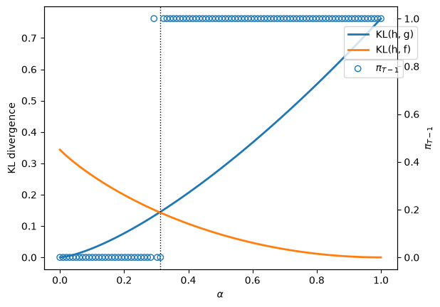
Fig. 32.5 Limit points and KL divergences#
values of α at which π_{T-1} lies on the side opposite to its limit: [0.293 0.313]
Evidently, our type 1 learner who applies Bayes’ law to his misspecified set of statistical models eventually learns an approximating model that is as close as possible to the true model, as measured by its Kullback-Leibler divergence:
When \(\alpha < \alpha^*\), \(KL_g < KL_f\), meaning the divergence of \(g\) from \(h\) is smaller than that of \(f\) and so the limit point of \(\pi_t\) is \(0\).
When \(\alpha > \alpha^*\), \(KL_f < KL_g\), meaning the divergence of \(f\) from \(h\) is smaller than that of \(g\) and so the limit point of \(\pi_t\) is \(1\).
For \(\alpha\) close to \(\alpha^*\), the drift \(KL_g(\alpha) - KL_f(\alpha)\) of \(\log L(w^t)\) is small relative to the standard deviation of \(\log \ell(w)\), and \(5000\) draws are too few to settle where \(\pi_t\) is going.
That is why the simulated values of \(\pi_{T-1}\) for the values of \(\alpha\) printed above, all near \(\alpha^*\), lie on the side opposite to the eventual limit.
32.6. Type 2 agent#
We now describe how our type 2 agent formulates his learning problem and what he eventually learns.
Our type 2 agent understands the correct statistical model but does not know \(\alpha\).
We apply Bayes’ law to deduce an algorithm for learning \(\alpha\) under the assumption that the agent knows that
but does not know \(\alpha\).
We’ll assume that the agent starts out with a prior probability density \(\pi_{-1}(\alpha)\) on \(\alpha \in (0,1)\) where the prior has one of the forms that we deployed in Non-Conjugate Priors.
We’ll fire up numpyro and apply it to the present situation.
Bayes’ law now takes the form
where \(\pi_t(\alpha)\) is the posterior density of \(\alpha\) given \(w^t\).
We’ll use numpyro to approximate this equation.
We’ll create graphs of the posterior \(\pi_t(\alpha)\) as \(t \rightarrow +\infty\) corresponding to ones presented in Non-Conjugate Priors.
We anticipate that a posterior distribution will collapse around the true \(\alpha\) as \(t \rightarrow + \infty\).
Let us try a uniform prior first.
We use the Mixture class in numpyro to construct the likelihood function.
α = 0.8
sizes = [5, 20, 50, 200, 1000, 25000]

# simulate data with true α
data = draw_lottery(jax.random.key(42), α, max(sizes))


def model(w):
    α = numpyro.sample("α", dist.Uniform(low=0.0, high=1.0))

    y_samp = numpyro.sample(
        "w",
        dist.Mixture(
            dist.Categorical(jnp.array([α, 1 - α])),
            [dist.Beta(F_a, F_b), dist.Beta(G_a, G_b)],
        ),
        obs=w,
    )


def MCMC_run(ws):
    "Compute posterior using MCMC with observed ws"

    kernel = NUTS(model)
    mcmc = MCMC(kernel, num_samples=5000, num_warmup=1000, progress_bar=False)

    mcmc.run(rng_key=random.key(42), w=jnp.array(ws))
    sample = mcmc.get_samples()
    return sample["α"]
The following code generates the graph below that displays Bayesian posteriors for \(\alpha\) at various history lengths.
fig, ax = plt.subplots()

for i in range(len(sizes)):
    sample = MCMC_run(data[: sizes[i]])
    sns.histplot(
        data=sample,
        kde=True,
        stat="density",
        alpha=0.2,
        ax=ax,
        color=colors[i],
        binwidth=0.02,
        linewidth=0.05,
        label=f"t={sizes[i]}",
    )
ax.legend()
ax.set_xlabel(r"$\alpha$")
plt.show()
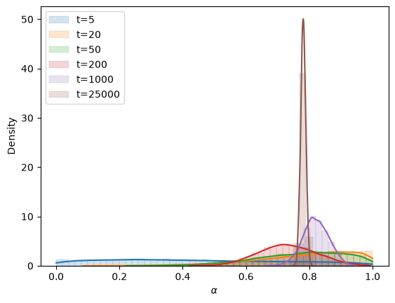
Fig. 32.6 Posterior for \(\alpha\) as \(t\) grows#
Evidently, the Bayesian posterior narrows in on the true value \(\alpha = 0.8\) of the mixing parameter as the length of a history of observations grows.
The posterior standard deviation shrinks in proportion to \(1/\sqrt{t}\); Exercise Exercise 32.3 computes the constant of proportionality.
32.7. Concluding remarks#
Our type 1 agent deploys an incorrect statistical model.
He believes that either \(f\) or \(g\) generated the \(w\) process, but just doesn’t know which one.
That is wrong because nature is actually mixing each period with mixing probability \(\alpha\).
Our type 1 agent eventually believes that either \(f\) or \(g\) generated the \(w\) sequence, the outcome being determined by the model, either \(f\) or \(g\), whose KL divergence relative to \(h\) is smaller.
At the knife-edge value \(\alpha^*\), the two divergences are equal and his beliefs never settle down.
Our type 2 agent has a different statistical model, one that is correctly specified.
He knows the parametric form of the statistical model but not the mixing parameter \(\alpha\).
He knows that he does not know it.
But by using Bayes’ law in conjunction with his statistical model and a history of data, he eventually acquires a more and more accurate inference about \(\alpha\).
This little laboratory exhibits some important general principles that govern outcomes of Bayesian learning of misspecified models.
Thus, the following situation prevails quite generally in empirical work.
A scientist approaches the data with a manifold \(S\) of statistical models \( s (X | \theta)\) , where \(s\) is a probability distribution over a random vector \(X\), \(\theta \in \Theta\) is a vector of parameters, and \(\Theta\) indexes the manifold of models.
The scientist with observations that he interprets as realizations \(x\) of the random vector \(X\) wants to solve an inverse problem of somehow inverting \(s(x | \theta)\) to infer \(\theta\) from \(x\).
But the scientist’s model is misspecified, being only an approximation to an unknown model \(h\) that nature uses to generate \(X\).
If the scientist uses Bayes’ law or a related likelihood-based method to infer \(\theta\) from IID observations, then for large sample sizes his inferences concentrate on values of \(\theta\) that minimize
over \(\theta \in \Theta\), where \(s_\theta = s(\cdot|\theta)\).
Berk [1966] established this for Bayesian posterior distributions, and White [1982] established it for maximum likelihood estimators.
When the minimizer \(\theta^*\) is unique, the posterior concentrates on \(\theta^*\) and the maximum likelihood estimator converges to \(\theta^*\).
When several values of \(\theta\) attain the minimum, the posterior concentrates on the set of minimizers but need not converge.
Our type 1 agent at \(\alpha = \alpha^*\) is an instance.
The section on KL divergence and maximum-likelihood estimation in Statistical Divergence Measures shows that maximum likelihood minimizes the cross-entropy of the model relative to the empirical distribution of the data, the sample analogue of the KL divergence from the data-generating distribution to the model.
Exercise Exercise 32.4 studies a type 2 agent whose model is misspecified.
32.8. Exercises#
Exercise 32.1
In Likelihood Ratio Processes and Bayesian Learning, we studied the consequences of applying a likelihood ratio and Bayes’ law to a misspecified statistical model, namely, our type 1 agent’s model, when the true data generating process is a mixture.
In this lecture, we used numpyro to compute posteriors of our type 2 agent, whose model is correctly specified.
This exercise asks you to replicate the type 2 agent’s posterior with a grid approximation and compare it with the NUTS posterior.
Here is the algorithm.
First we specify a prior distribution for \(\alpha\) given by \(\alpha \sim \mathrm{Beta}(a_0, b_0)\) with expectation \(\mathbb{E}[\alpha] = \frac{a_0}{a_0 + b_0}\).
The likelihood for a single observation \(w_t\) is \(h(w_t|\alpha) = \alpha f(w_t) + (1-\alpha) g(w_t)\).
For a history \(w^t = (w_0, \dots, w_t)\), the likelihood is \(\prod_{s=0}^t h(w_s|\alpha)\).
The posterior density is \(\pi_t(\alpha) \propto \prod_{s=0}^t h(w_s|\alpha) \pi_{-1}(\alpha)\).
Recursively, \(\pi_t(\alpha) \propto h(w_t|\alpha) \pi_{t-1}(\alpha)\).
Without a conjugate prior, we can approximate the posterior by discretizing \(\alpha\) into a grid.
Implement this algorithm in Python.
With a uniform prior (\(a_0 = b_0 = 1\)), compute the posterior of \(\alpha\) from the first \(5, 20, 50, 200\), and \(1000\) observations in
dataand compare it with the NUTS posterior.Let the true mixing probability be \(\alpha = 0.5\). For a history of \(200\) draws, compute the paths of posterior means of \(\alpha\) for three priors with means \(0.25\), \(0.5\), and \(0.75\). Then compute paths of posterior means with a uniform prior for \(20\) histories of \(10{,}000\) draws.
Solution
Here is one solution.
We put a grid on \(\alpha\) and update the log posterior on the grid one observation at a time.
α_grid = jnp.linspace(1e-3, 1 - 1e-3, 2000)
Δα = float(α_grid[1] - α_grid[0])


@jax.jit
def learn_α_bayesian(observations, a0, b0):
    """
    Sequential Bayesian learning of the mixing probability α on α_grid.
    Returns the path of posterior means, starting from the prior mean,
    and the final log posterior probabilities on the grid.
    """
    w = jnp.asarray(observations)

    # Log prior
    log_prior = (a0 - 1) * jnp.log(α_grid) + (b0 - 1) * jnp.log1p(-α_grid)
    log_prior = log_prior - jax.nn.logsumexp(log_prior)

    def scan_fn(log_post, wt):
        # h(w_t | α) = α f(w_t) + (1 - α) g(w_t)
        like = α_grid * f(wt) + (1 - α_grid) * g(wt)
        log_post = log_post + jnp.log(like)

        # Normalize using log-sum-exp trick
        log_post = log_post - jax.nn.logsumexp(log_post)

        # Compute posterior mean
        μ = α_grid @ jnp.exp(log_post)

        return log_post, μ

    # Scan over observations
    log_post, μ_path = jax.lax.scan(scan_fn, log_prior, w)

    # Prepend the prior mean
    μ_prior = a0 / (a0 + b0)
    return jnp.concatenate([jnp.array([μ_prior]), μ_path]), log_post
Now we compare the grid posterior densities with the NUTS draws for the data used in the lecture.
fig, ax = plt.subplots()

for i, n in enumerate(sizes[:-1]):
    _, log_post = learn_α_bayesian(data[:n], 1.0, 1.0)
    density = np.exp(log_post) / Δα
    sample = MCMC_run(data[:n])
    ax.hist(np.asarray(sample), bins=50, density=True, alpha=0.3,
            color=colors[i], label=f"NUTS, t={n}")
    ax.plot(α_grid, density, color=colors[i], lw=2)
    print(f"t = {n:4d}: grid mean = {float(α_grid @ jnp.exp(log_post)):.4f}, "
          f"NUTS mean = {float(sample.mean()):.4f}")

ax.set_xlabel(r"$\alpha$")
ax.legend()
plt.show()
t =    5: grid mean = 0.4568, NUTS mean = 0.4487
t =   20: grid mean = 0.7885, NUTS mean = 0.7897
t =   50: grid mean = 0.7753, NUTS mean = 0.7737
t =  200: grid mean = 0.7318, NUTS mean = 0.7302
t = 1000: grid mean = 0.8216, NUTS mean = 0.8206
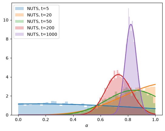
The lines are the grid posteriors and the histograms are the NUTS draws.
They agree up to Monte Carlo error in the NUTS draws.
Next we study the paths of posterior means for three priors when \(\alpha = 0.5\).
α_true = 0.5
T_mix = 200

# Three different priors with means 0.25, 0.5, 0.75
prior_params = [(1, 3), (1, 1), (3, 1)]
prior_means = [a0 / (a0 + b0) for a0, b0 in prior_params]

w_mix = draw_lottery(jax.random.key(42), α_true, T_mix)

α_posterior_means = [learn_α_bayesian(w_mix, float(a0), float(b0))[0]
                     for a0, b0 in prior_params]
Let’s visualize how the posterior mean of \(\alpha\) evolves over time, starting from three different prior beliefs.
fig, ax = plt.subplots()

for i, (α_means, mean0) in enumerate(zip(α_posterior_means, prior_means)):
    ax.plot(
        range(-1, T_mix),
        α_means,
        label=rf"Prior mean = ${mean0:.2f}$",
        color=colors[i],
        linewidth=2,
    )

ax.axhline(
    y=α_true,
    color="black",
    linestyle="--",
    label=rf"True $\alpha$ = {α_true}",
    linewidth=2,
)
ax.set_xlabel("$t$")
ax.set_ylabel(r"Posterior mean of $\alpha$")
ax.legend()
plt.show()

for α_means, mean0 in zip(α_posterior_means, prior_means):
    print(f"prior mean {mean0:.2f}: posterior mean at t = {T_mix - 1} is {float(α_means[-1]):.3f}")
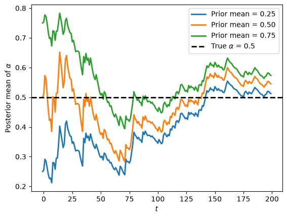
prior mean 0.25: posterior mean at t = 199 is 0.512
prior mean 0.50: posterior mean at t = 199 is 0.545
prior mean 0.75: posterior mean at t = 199 is 0.573
All three posterior means move toward the true value \(\alpha = 0.5\), and their differences shrink as \(t\) grows.
Next, let’s look at multiple simulations with a longer time horizon, all starting from a uniform prior.
n_paths = 20
T_long = 10_000

keys = jax.random.split(jax.random.key(42), n_paths)

fig, ax = plt.subplots()

for j in range(n_paths):
    w_path = draw_lottery(keys[j], α_true, T_long)
    α_means, _ = learn_α_bayesian(w_path, 1.0, 1.0)  # Uniform prior
    ax.plot(range(-1, T_long), α_means, alpha=0.5, lw=2)

ax.axhline(
    y=α_true,
    color="red",
    linestyle="--",
    label=rf"True $\alpha$ = {α_true}",
    linewidth=2,
)
ax.set_ylabel(r"Posterior mean of $\alpha$")
ax.set_xlabel("$t$")
ax.legend()
plt.tight_layout()
plt.show()
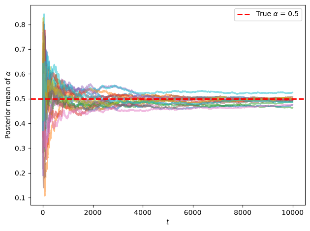
We can see that the posterior mean of \(\alpha\) converges to the true value \(\alpha = 0.5\).
Exercise 32.2
This exercise studies the type 1 agent at the knife-edge value \(\alpha^*\).
Compute \(\alpha^*\) by finding the root of \(KL_f(\alpha) - KL_g(\alpha)\) and compare it with the formula \(\alpha^* = KL(g, f)/(KL(f, g) + KL(g, f))\).
For \(\alpha \in \{\alpha^* - 0.05, \alpha^*, \alpha^* + 0.05\}\), simulate \(20\) paths of \(\log L(w^t)\) for \(t = 0, \ldots, 19{,}999\) and plot them.
For each \(\alpha\), compute \(\pi_t\) from (32.3) with \(\pi_{-1} = 0.5\), and count how often each path of \(\pi_t\) crosses \(1/2\) during the second half of the sample.
Solution
We compute \(KL_f\) and \(KL_g\) with quad and find their crossing with brentq.
def KL_h(α, q):
    "KL(h, q) for h = h(·|α), computed with quad."
    h = lambda w: α * f(w) + (1 - α) * g(w)
    return KL(h, q)

α_root = brentq(lambda α: KL_h(α, f) - KL_h(α, g), 0.05, 0.95)
print(f"root of KL_f - KL_g: {α_root:.5f}")
print(f"formula:             {α_star:.5f}")
root of KL_f - KL_g: 0.31156
formula:             0.31156
Next we simulate paths of \(\log L(w^t)\).
T_k, N_k = 20_000, 20
α_values = [α_star - 0.05, α_star, α_star + 0.05]

fig, axes = plt.subplots(1, 3, figsize=(14, 4), sharey=True)
for ax, α_k, key in zip(axes, α_values, jax.random.split(jax.random.key(1), 3)):
    log_L = np.cumsum(np.log(np.asarray(simulate_mixed(key, α_k, T=T_k, N=N_k))), axis=1)
    ax.plot(log_L.T, lw=1, alpha=0.6)
    ax.axhline(0, color='k', lw=1)
    ax.set_title(rf"$\alpha = {α_k:.3f}$")
    ax.set_xlabel("$t$")

    π_paths = expit(log_L)            # π_{-1} = 0.5, so the prior log odds are zero
    late = π_paths[:, T_k // 2:] > 0.5
    crossings = np.sum(late[:, 1:] != late[:, :-1], axis=1)
    print(f"α = {α_k:.3f}: crossings of 1/2 in second half, by path: {crossings}")

axes[0].set_ylabel(r"$\log L(w^t)$")
plt.tight_layout()
plt.show()
α = 0.262: crossings of 1/2 in second half, by path: [0 0 0 0 0 0 0 0 0 0 0 0 0 0 0 0 0 0 0 0]
α = 0.312: crossings of 1/2 in second half, by path: [58 14 11  0 63 44  0 12 23 39  0  0 41  0  0  0  0 93  0 42]
α = 0.362: crossings of 1/2 in second half, by path: [0 0 0 0 0 0 0 0 0 0 0 0 0 0 0 0 0 0 0 0]
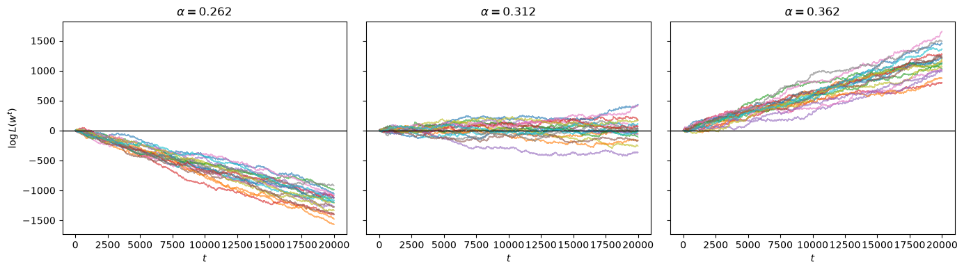
At \(\alpha^* \pm 0.05\), every path of \(\log L(w^t)\) drifts away from zero and \(\pi_t\) stops crossing \(1/2\).
At \(\alpha^*\), the paths wander without drift, and many paths of \(\pi_t\) still cross \(1/2\) late in the sample.
A path that does not cross \(1/2\) during the second half is not evidence of convergence.
A driftless random walk spends long stretches on one side of zero, and with probability one it returns.
Exercise 32.3
The Bernstein–von Mises theorem says that, for a correctly specified model, the posterior distribution of \(\alpha\) after \(t\) observations is approximately normal with mean near the true \(\alpha\) and standard deviation \(1/\sqrt{t I(\alpha)}\), where
is the Fisher information of one observation.
Derive \(I(\alpha)\) from the log likelihood \(\log h(w|\alpha)\).
For the data in
data(\(\alpha = 0.8\)), compute the grid posterior standard deviation after \(200\), \(1000\), and \(5000\) observations with a uniform prior, and compare it with \(1/\sqrt{t I(0.8)}\).
Solution
The score of one observation is \(\frac{\partial}{\partial \alpha} \log h(w|\alpha) = \frac{f(w) - g(w)}{h(w|\alpha)}\).
Its variance under \(h(\cdot|\alpha)\) is the Fisher information
because the score has mean \(\int (f - g) dw = 0\).
def fisher_info(α):
    return quad(lambda w: (f(w) - g(w))**2 / (α * f(w) + (1 - α) * g(w)), 0, 1)[0]

I_08 = fisher_info(0.8)
print(f"I(0.8) = {I_08:.4f}")

for n in [200, 1000, 5000]:
    _, log_post = learn_α_bayesian(data[:n], 1.0, 1.0)
    post = jnp.exp(log_post)
    mean = α_grid @ post
    sd = jnp.sqrt(((α_grid - mean)**2) @ post)
    print(f"t = {n:4d}: posterior mean = {float(mean):.3f}, posterior sd = {float(sd):.4f}, "
          f"1/sqrt(t I) = {1 / np.sqrt(n * I_08):.4f}")
I(0.8) = 0.5835
t =  200: posterior mean = 0.732, posterior sd = 0.0925, 1/sqrt(t I) = 0.0926
t = 1000: posterior mean = 0.822, posterior sd = 0.0418, 1/sqrt(t I) = 0.0414
t = 5000: posterior mean = 0.787, posterior sd = 0.0186, 1/sqrt(t I) = 0.0185
The posterior standard deviations are close to \(1/\sqrt{t I(0.8)}\).
Exercise 32.4
Suppose that nature draws IID from \(h(w|0.5) = 0.5 f(w) + 0.5 g(w)\) with \(g = \) Beta\((3, 1.2)\), as in the lecture.
A type 2 agent knows \(f\) but wrongly believes that the second component is \(\tilde g = \) Beta\((3, 2)\).
His model is \(s(w|\alpha) = \alpha f(w) + (1-\alpha) \tilde g(w)\), and he puts a uniform prior on \(\alpha\).
Compute \(\tilde \alpha = \arg\min_\alpha KL(h, s_\alpha)\).
Simulate \(5000\) draws from \(h(\cdot|0.5)\) and compute the agent’s grid posterior after \(200\), \(1000\), and \(5000\) observations. Where does it concentrate?
Solution
g_tilde = jax.jit(lambda x: p(x, 3, 2))
α_true = 0.5
h_true = lambda w: α_true * f(w) + (1 - α_true) * g(w)

def KL_misspecified(α):
    s = lambda w: α * f(w) + (1 - α) * g_tilde(w)
    return KL(h_true, s)

res = minimize_scalar(KL_misspecified, bounds=(1e-3, 1 - 1e-3), method='bounded')
α_tilde = res.x
print(f"pseudo-true value α~ = {α_tilde:.3f}, min KL = {res.fun:.4f}")
pseudo-true value α~ = 0.616, min KL = 0.0460
The agent’s grid posterior uses \(\tilde g\) in place of \(g\).
@jax.jit
def log_post_misspecified(observations):
    "Log posterior on α_grid, uniform prior, for the model α f + (1 - α) g~."
    w = jnp.asarray(observations)
    log_like = jnp.log(α_grid[:, None] * f(w) + (1 - α_grid[:, None]) * g_tilde(w))
    log_post = jnp.sum(log_like, axis=1)
    return log_post - jax.nn.logsumexp(log_post)

w_obs = draw_lottery(jax.random.key(7), α_true, 5000)

fig, ax = plt.subplots()
for i, n in enumerate([200, 1000, 5000]):
    post = jnp.exp(log_post_misspecified(w_obs[:n]))
    mean = float(α_grid @ post)
    sd = float(jnp.sqrt(((α_grid - mean)**2) @ post))
    ax.plot(α_grid, post / Δα, color=colors[i], lw=2, label=f"t={n}")
    print(f"t = {n:4d}: posterior mean = {mean:.3f}, posterior sd = {sd:.4f}")

ax.axvline(α_true, color="k", linestyle="--", label=r"true $\alpha$")
ax.axvline(α_tilde, color="r", linestyle=":", label=r"$\tilde \alpha$")
ax.set_xlabel(r"$\alpha$")
ax.legend()
plt.show()
t =  200: posterior mean = 0.701, posterior sd = 0.1066
t = 1000: posterior mean = 0.663, posterior sd = 0.0493
t = 5000: posterior mean = 0.619, posterior sd = 0.0218
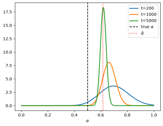
The posterior concentrates at the pseudo-true value \(\tilde \alpha\), not at the true \(\alpha = 0.5\).
As Berk [1966] showed, a Bayesian with a misspecified model learns the member of his family of models that is closest to the truth in Kullback–Leibler divergence.