104. Escaping Nash Inflation#
104.1. Overview#
If an unlikely event occurs, it is very likely to occur in the most likely way.
– Michael Harrison
This lecture is the analytical companion to Adaptive Learning and Escape Dynamics.
It follows Cho et al. [2002] (CWS), who give a deterministic characterization of the escape dynamics that chapter 8 of Sargent [1999] found by simulation.
In Adaptive Learning and Escape Dynamics we watched a constant-gain government recurrently escape the Nash self-confirming equilibrium and spend long spells near the Ramsey outcome, but we described those escapes only informally and by simulation.
CWS show that the escapes are governed by their own ordinary differential equation, obtained from the theory of large deviations.
The picture that emerges has two deterministic pieces:
the mean dynamics, an ODE that pulls the government’s beliefs toward the self-confirming equilibrium; and
the escape dynamics, a second ODE that, driven by a “most likely unlikely” sequence of shocks, pushes beliefs away from it, toward the beliefs that support the Ramsey outcome.
The remarkable finding is that the escape has a dominant path: conditional on escaping, the government’s beliefs follow a nearly deterministic route along which it temporarily learns a version of the natural-rate hypothesis and cuts inflation.
These escapes recur because the government uses constant-gain least squares, as in Sargent [1999] and CWS.
The governments of Sims [1988] and Chung [1990] instead ran Kalman filters on drifting coefficients; in their simulations a government that escaped did so once and then stayed near Ramsey, apparently indefinitely, and Priors, Escapes, and Learning Cycles traces the difference to the government’s prior.
The large-deviation results are statements about small gains.
Simulating escapes simulates the model and finds that, at the gains used in this suite, escapes are frequent rather than rare.
We work with the analytically tractable static model, in which the government regresses unemployment on current inflation and a constant.
Adaptive Learning and Escape Dynamics simulates CWS’s richer dynamic model, in which the government’s regression also includes lags; we compare the two near the end of the lecture.
A government learning the Phillips curve presents the same static model, with the same calibration, in condensed form.
Readers arriving from there should note that it writes the beliefs as \(\alpha\) (intercept first) and the gain as \(\gamma\), while here \(\gamma\) denotes the beliefs and \(\varepsilon\) the gain.
The next lecture, Priors, Escapes, and Learning Cycles, asks how the government’s prior about parameter drift reshapes both the mean dynamics and the escape dynamics.
Let’s start with our imports:
import matplotlib.pyplot as plt
import numpy as np
from scipy.integrate import solve_ivp
from scipy.linalg import solve_discrete_are
104.2. The model#
The true economy is the natural-rate model of Kydland and Prescott [1977],
with \(\theta, u > 0\) and \(W_n = (W_{1n}, W_{2n})^\top\) IID standard Gaussian.
The government does not know (104.1).
In the static model it fits a non-expectational Phillips curve by regressing unemployment on inflation and a constant,
with beliefs \(\gamma = (\gamma_1, \gamma_{-1})\) (slope and intercept), and it treats \(\eta_n\) as exogenous.
Note
We keep the ordering of Cho et al. [2002]: the slope comes first, and the regressors are \(\Phi = (\pi, 1)\).
This also matches the \(\gamma_1, \gamma_{-1}\) convention of Self-Confirming Equilibria.
Priors, Escapes, and Learning Cycles and A government learning the Phillips curve follow Sargent and Williams [2005] and put the intercept first.
Each lecture follows its source paper; the warning box in Priors, Escapes, and Learning Cycles translates between the two.
Believing (104.2), the government solves the Phelps problem, whose static best response sets inflation to the constant
Three beliefs are worth naming, following CWS:
Belief 1 (Nash): \(\gamma_1 = -\theta\) with an intercept that makes \(x = \theta u\), the time-consistent outcome of Kydland and Prescott [1977].
Belief 2 (Ramsey): \(\gamma_1 = 0\), so the government perceives no tradeoff and sets \(x = 0\).
Belief 3 (induction): in CWS’s dynamic model, coefficients on current and lagged inflation that sum to zero, which for a patient government also sends inflation to \(0\).
In the static model there is only one coefficient on inflation, so Belief 3 coincides with Belief 2: a vertical perceived Phillips curve “trivially satisfies the induction property” (CWS, section 6.2).
class EscapeModel:
    "CWS 2002 static model. γ = (γ₁ slope, γ₋₁ intercept), regressors Φ = (π, 1)."

    def __init__(self, θ=1.0, u=5.0, σ1=0.3, σ2=0.3):
        self.θ, self.u, self.σ1, self.σ2 = θ, u, σ1, σ2

    def γ_sce(self):
        "Self-confirming beliefs (slope -θ, intercept u(1+θ²))."
        return np.array([-self.θ, self.u * (1 + self.θ**2)])

    def x(self, γ):
        γ1, γm1 = γ
        return -γm1 * γ1 / (1 + γ1**2)

    def M(self, γ):
        "E[ΦΦ'] with Φ = (π, 1)."
        x = self.x(γ)
        return np.array([[x**2 + self.σ2**2, x], [x, 1.0]])

    def g_bar(self, γ):
        "Mean-dynamics forcing E[Φ(U − Φ'γ)] = M(T(γ) − γ)."
        x = self.x(γ)
        E_ΦU = np.array([x * self.u - self.θ * self.σ2**2, self.u])
        return E_ΦU - self.M(γ) @ γ
104.3. The self-confirming equilibrium#
A self-confirming equilibrium is a belief that reproduces itself: the population regression coefficients of (104.2), computed on the data the government generates by acting on \(\gamma\), equal \(\gamma\).
Writing \(T(\gamma)\) for those population coefficients and \(\bar M(\gamma) = \mathbb{E}\,\Phi\Phi^\top\) for the population moment matrix of the regressors, CWS show
so a self-confirming equilibrium solves \(\bar g(\gamma) = 0\).
Under a constant policy \(x\), only the surprise \(\sigma_2 W_{2n}\) moves inflation, so \(T(\gamma) = (-\theta,\ u + \theta x(\gamma))\).
For the static model the equilibrium is therefore the intersection of the line \(\gamma_1 = -\theta\) with the parabola \(\gamma_{-1} = u(1 + \gamma_1^2)\), a unique point that supports the Nash outcome of The Credibility Problem.
It is the same self-confirming equilibrium constructed in Self-Confirming Equilibria, written here in the static (constant-plus-slope) special case that Priors, Escapes, and Learning Cycles also uses, and it is what Kydland and Prescott [1977] call a consistent equilibrium (A government learning the Phillips curve).
model = EscapeModel(θ=1.0, u=5.0, σ1=0.3, σ2=0.3)
γ_sce = model.γ_sce()

print(f"self-confirming beliefs γ = {γ_sce}  (slope -θ, intercept u(1+θ²))")
print(f"self-confirming inflation x = {model.x(γ_sce):.2f}  (= Nash = θu)")
print(f"check g_bar = {model.g_bar(γ_sce)}")
self-confirming beliefs γ = [-1. 10.]  (slope -θ, intercept u(1+θ²))
self-confirming inflation x = 5.00  (= Nash = θu)
check g_bar = [0. 0.]
The figure plots the two loci whose intersection is the equilibrium.
γ1_grid = np.linspace(-2, 1, 200)
fig, ax = plt.subplots(figsize=(7, 6))
ax.plot(γ1_grid, model.u * (1 + γ1_grid**2), label=r'$\gamma_{-1} = u(1+\gamma_1^2)$', lw=2)
ax.axvline(-model.θ, color='C1', ls='--', label=r'$\gamma_1 = -\theta$')
ax.plot(γ_sce[0], γ_sce[1], 'ko', ms=8)
ax.annotate('SCE (Nash)', γ_sce, (γ_sce[0] + 0.1, γ_sce[1] + 1))
ax.set_xlabel(r'slope $\gamma_1$')
ax.set_ylabel(r'intercept $\gamma_{-1}$')
ax.set_ylim(0, 25)
ax.legend()
plt.show()
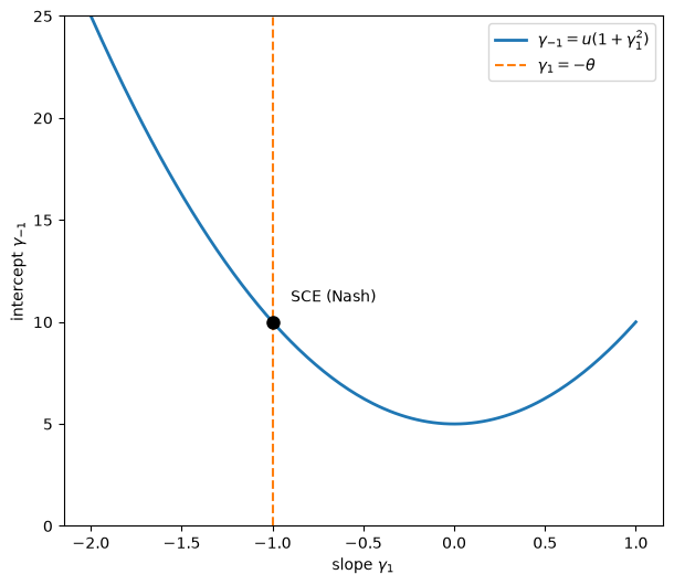
Fig. 104.1 The unique self-confirming equilibrium in belief space#
104.4. Adaptation and the mean dynamics#
We make the government adaptive.
Each period it sets \(x_n = x(\gamma_n)\), observes \((\pi_n, U_n)\), and updates its estimates by constant-gain recursive least squares,
where \(\Phi_n = (\pi_n, 1)^\top\) and \(\varepsilon > 0\) is the gain.
This is the recursion of constant_gain in A government learning the Phillips curve, with the regressors in CWS’s order.
CWS’s equations (4.24)–(4.25) date \(R\) one period earlier, which makes no difference as \(\varepsilon \to 0\).
Because the government acts on its current estimate as if it were permanent, this is an anticipated-utility model in the sense of Kreps [1998].
The literature on least squares learning in self-referential models [Evans and Honkapohja, 2001, Marcet and Sargent, 1989, Woodford, 1990] shows that, as \(\varepsilon \to 0\) with time measured as \(t = n\varepsilon\), the beliefs are approximated by the mean-dynamics ODE
One recursion, many learners derives this kind of ODE for a scalar recursion and connects its stability to E-stability.
Note
Notation across lectures. A primer on recursive algorithms stacks the beliefs as \(\phi = (\gamma, \operatorname{col}(R))\) and writes the mean dynamics as \(\dot\phi = b(\phi)\).
In the static model \(b(\phi) = \left(R^{-1}\bar g(\gamma),\ \operatorname{col}(\bar M(\gamma) - R)\right)\), so (104.5) is that ODE written out.
The escape dynamics below add a forcing \(v\) to the \(\gamma\) block only.
Priors, Escapes, and Learning Cycles replaces the scaled inverse moment matrix \(\varepsilon R^{-1}\) by the covariance matrix \(P\) of a Kalman filter, and orders \(\gamma\) intercept first.
A rest point of (104.5) is a self-confirming equilibrium, and CWS show that this ODE is globally stable about it.
Locally, with \(R = \bar M(\bar\gamma)\), the \(\gamma\) block has eigenvalues \(-1\) and \(-1/(1+\theta^2)\): these are the E-stability eigenvalues of Uniqueness and E-stability and Mean dynamics near the self-confirming equilibrium.
R_bar = model.M(γ_sce)                     # moment matrix at the SCE
h = 1e-6
J = np.column_stack([(model.g_bar(γ_sce + h * e) - model.g_bar(γ_sce - h * e)) / (2 * h)
                     for e in np.eye(2)])
print("eigenvalues of R̄⁻¹ Dḡ at the SCE:", np.linalg.eigvals(np.linalg.solve(R_bar, J)).round(4))
print("-1/(1+θ²) =", -1 / (1 + model.θ**2))
eigenvalues of R̄⁻¹ Dḡ at the SCE: [-1.  -0.5]
-1/(1+θ²) = -0.5
So under the mean dynamics alone, the adaptive government is drawn to Nash inflation.
But the route can be circuitous.
The next figure starts the beliefs part of the way toward Ramsey, at \(\gamma(0) = \bar\gamma + (0.4, -3)\), in two ways.
In the first, the moment matrix \(R\) starts at its Nash-era value \(\bar M(\bar\gamma)\); in the second, it starts at the moments \(\bar M(\gamma(0))\) that the new beliefs would generate.
def mean_ode(t, z, model):
    γ, R = z[:2], z[2:].reshape(2, 2)
    return np.concatenate([np.linalg.solve(R, model.g_bar(γ)),
                           (model.M(γ) - R).ravel()])

γ0 = γ_sce + np.array([0.4, -3.0])
fig, ax = plt.subplots(figsize=(8, 4.5))
starts = [(R_bar, r'$R(0) = \bar M(\bar\gamma)$ (Nash-era moments)', 'R(0) = M(SCE)'),
          (model.M(γ0), r'$R(0) = \bar M(\gamma(0))$', 'R(0) = M(γ(0))')]
for R0, label, short in starts:
    sol = solve_ivp(mean_ode, [0, 60], np.concatenate([γ0, R0.ravel()]), args=(model,),
                    max_step=0.1, rtol=1e-9, atol=1e-11)
    x_path = -sol.y[1] * sol.y[0] / (1 + sol.y[0]**2)
    ax.plot(sol.t, x_path, label=label)
    k = np.argmin(x_path)
    print(f"{short:15s}: x(0) = {x_path[0]:.2f}, min x = {x_path[k]:.2f} "
          f"at t = {sol.t[k]:.2f}, x(60) = {x_path[-1]:.2f}")
ax.axhline(model.θ * model.u, color='k', ls='--', lw=1, label='Nash')
ax.set_xlabel('time $t = n\\varepsilon$')
ax.set_ylabel('inflation $x$')
ax.legend()
plt.show()
R(0) = M(SCE)  : x(0) = 3.09, min x = 1.68 at t = 1.33, x(60) = 5.00
R(0) = M(γ(0)) : x(0) = 3.09, min x = 3.09 at t = 0.00, x(60) = 5.00
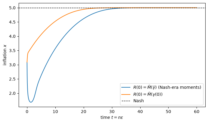
Fig. 104.2 Mean dynamics from a perturbed start: when R starts at its Nash-era value, inflation first dips#
Both paths return to Nash, but they get there differently.
When \(R\) starts at the Nash-era moments, inflation first falls further, from about 3.1 to about 1.7, before it climbs back.
When \(R\) starts at \(\bar M(\gamma(0))\), inflation rises monotonically.
The dip is the circuitous route of CWS (section 6.4) made visible, and it comes from \(R\) lagging behind \(\bar M(\gamma)\).
We return to this lag in Mean dynamics reinforce the escape, where it turns out to drive the escape.
The mean dynamics alone cannot explain the recurrent visits to low inflation in the simulations of Adaptive Learning and Escape Dynamics.
For that we need a second force.
104.5. Escape dynamics as a control problem#
Although the impact of the noise vanishes as \(\varepsilon \to 0\), for a fixed positive gain unusual sequences of shocks can push beliefs a long way from the self-confirming equilibrium.
A primer on recursive algorithms sets out the general theory.
It builds the log moment-generating function \(H\) of the innovations, its Legendre transform \(L\), and an action functional \(S(T, \gamma) = \int_0^T L\, ds\) that measures how improbable a path of beliefs is.
The dominant escape path minimizes the action among paths that leave a neighbourhood \(G\) of \(\bar\gamma\).
Here we need only the operational version.
CWS draw on Noah Williams’s dissertation [Williams, 2001], published in corrected form as Williams [2019], to reduce the problem to a clean control problem.
The H-functional becomes a quadratic form with a normalizing matrix \(Q\) (a fourth-moment matrix obtained from Lyapunov equations), and the escape path solves
subject to the perturbed mean dynamics
Read (104.6) as a least squares problem: \(v\) is the extra “forcing” that the mean dynamics would need to escape, \(Q\) plays the role of a covariance matrix, and the least-cost forcing is the most likely unusual shock sequence.
Williams [2019] (p. 892) reports that the 2001 version computed \(H\) by misapplying a theorem of Worms (1999).
The discrepancy matters only for dynamic models; for the static model CWS computed \(H\) directly.
So the static-model results below stand, while CWS’s rate for the dynamic model rests on the earlier shortcut.
Let \(\tau^\varepsilon\) be the first time, measured as \(t = n\varepsilon\), at which the beliefs leave \(G\).
Two consequences (CWS, Theorem 5.3) tie the control problem to the stochastic model:
\(\varepsilon \log \mathbb{P}(\text{escape before } T) \to -\bar S\) and \(\varepsilon \log \mathbb{E}\,\tau^\varepsilon \to \bar S\) as \(\varepsilon \to 0\); and
conditional on escaping, beliefs follow the dominant escape path with probability approaching one.
The first is a statement about the limit \(\varepsilon \to 0\).
Williams [2019] (footnote 16) writes it as \(\log \mathbb{E}\,\tau^\varepsilon \approx S_0 + \bar S/\varepsilon\) for some constant \(S_0\) that the theory does not pin down.
So \(\bar S\) governs how fast escape times grow as the gain shrinks, not their level.
For the static model CWS (Table 1) find \(\bar S \approx 5 \times 10^{-4}\).
At the gains of Adaptive Learning and Escape Dynamics and A government learning the Phillips curve (0.025 and 0.02), \(e^{\bar S/\varepsilon} \approx 1.02\), so the large-deviation factor by itself does not make escapes rare.
Simulating escapes measures how often they occur.
The escape dynamics, like the mean dynamics, are deterministic.
104.6. The changed-measure escape path#
Solving (104.6) requires the matrix \(Q\) and a two-point boundary-value problem.
For the static model with binomial shocks, CWS (section 7) identify the escape route by a different and simpler argument.
They change the probability measure on the shocks to the most likely unusual distribution that pushes beliefs away from \(\bar\gamma\), and average the least squares update under that measure.
The resulting escape forcing is strikingly simple:
so the changed-measure escape path solves
This path shares the dominant escape path’s exit point, but it gets there faster.
CWS (footnote 14) warn that the transformed measure underestimates the time to escape.
In their Figure 7, the changed-measure path is shorter than even the shortest of 1,000 simulated escapes.
Let’s integrate (104.9) from the self-confirming equilibrium until beliefs leave a circle of radius 5, the escape set CWS use for the static model.
def escape_ode(t, z, model):
    γ, R = z[:2], z[2:].reshape(2, 2)
    force = np.array([model.σ1 * model.σ2, 0.0])
    return np.concatenate([np.linalg.solve(R, model.g_bar(γ) + force),
                           (model.M(γ) - R).ravel()])

def left_circle(t, z, *args):
    "Terminal event: beliefs leave the radius-5 circle around the SCE."
    return 5.0 - np.linalg.norm(z[:2] - γ_sce)
left_circle.terminal = True
left_circle.direction = -1

z0 = np.concatenate([γ_sce, R_bar.ravel()])
esc = solve_ivp(lambda t, z: escape_ode(t, z, model), [0, 200], z0,
                events=left_circle, max_step=0.02, rtol=1e-9, atol=1e-11)

slope, intercept = esc.y[0], esc.y[1]
infl = -intercept * slope / (1 + slope**2)
The figure plots the two coefficients and the inflation rate they imply.
fig, axes = plt.subplots(1, 2, figsize=(12, 5))

axes[0].plot(esc.t, intercept, label='intercept $\\gamma_{-1}$')
axes[0].plot(esc.t, slope, label='slope $\\gamma_1$')
axes[0].axhline(0, color='C3', ls=':', lw=1, label='vertical curve ($\\gamma_1 = 0$)')
axes[0].set_xlabel('time $t = n\\varepsilon$')
axes[0].set_ylabel('coefficient')
axes[0].set_title('Changed-measure escape path (cf. CWS Figures 4 and 7)')
axes[0].legend()

axes[1].plot(esc.t, infl)
axes[1].axhline(model.θ * model.u, color='k', ls='--', lw=1, label='Nash')
axes[1].axhline(0, color='C2', ls=':', lw=1, label='Ramsey')
axes[1].set_xlabel('time $t = n\\varepsilon$')
axes[1].set_ylabel('inflation $x$')
axes[1].set_title('Inflation along the escape')
axes[1].legend()

plt.tight_layout()
plt.show()
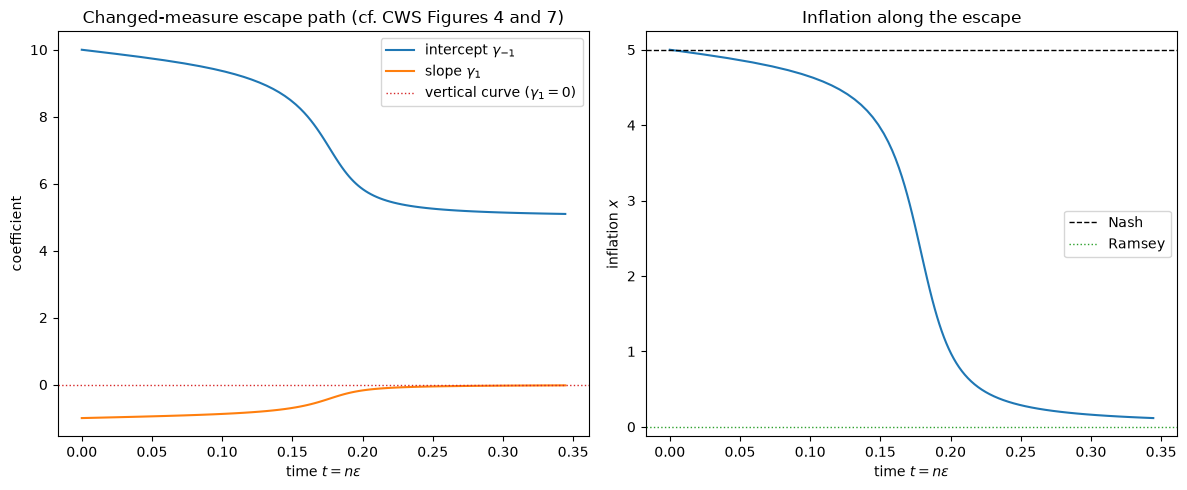
Fig. 104.3 The changed-measure escape path and the inflation rate along it#
Here are the start and end points of the path.
print(f"exit time : t = {esc.t[-1]:.3f}")
print(f"slope     : {slope[0]:.2f} → {slope[-1]:.3f}   (CWS Table 1, radius 5: -0.025)")
print(f"intercept : {intercept[0]:.1f} → {intercept[-1]:.2f}")
print(f"inflation : {infl[0]:.2f} → {infl[-1]:.2f}   (Nash {model.θ*model.u:.0f} → Ramsey 0)")
exit time : t = 0.344
slope     : -1.00 → -0.023   (CWS Table 1, radius 5: -0.025)
intercept : 10.0 → 5.10
inflation : 5.00 → 0.12   (Nash 5 → Ramsey 0)
Along the escape path the slope rises from its self-confirming value of \(-1\) toward zero, and inflation falls from the Nash value toward Ramsey.
The path leaves the circle at a slope of about \(-0.023\), close to the \(-0.025\) that CWS (Table 1) report for the dominant path at the same radius.
It leaves at \(t \approx 0.34\), while the dominant path in CWS’s Figure 4 needs until about \(t = 3\): the two paths share a route but not a timetable.
In the static model, a slope near zero means a vertical perceived Phillips curve, which trivially satisfies the induction hypothesis.
The dynamic model that Adaptive Learning and Escape Dynamics simulates escapes differently.
There the sum of the coefficients on current and lagged inflation rises toward zero, while the coefficient on current inflation stays negative, so a short-run Phillips curve survives while the long-run curve becomes vertical (CWS, section 6.2 and Figure 3).
In both models the government, by chance, generates enough inflation experiments to discover a good-enough version of the natural-rate hypothesis, and acts on it.
104.7. The race of four ODEs#
Where does the escape forcing (104.8) come from?
With binomial shocks \(W_{in} \in \{-1, +1\}\), each period brings one of four shock realizations \(w \in \{-1, 1\}^2\), each with probability \(1/4\).
An escape needs a run of updates that push beliefs consistently in one direction.
CWS show that the most efficient runs draw repeatedly from just two realizations whose updates lie in the same half-space, each with probability \(1/2\); four such pairs exist.
Averaging the update over a pair gives a conditional mean ODE,
with forcings
for the pairs \(\{(1,1), (-1,-1)\}\), \(\{(1,-1), (-1,1)\}\), \(\{(1,1), (1,-1)\}\) and \(\{(-1,1), (-1,-1)\}\).
\(R\) follows the unconditional mean dynamics because \(\bar M\) depends only on \(W_2\), which takes each value with probability \(1/2\) within every pair.
Each conditional ODE is a candidate escape route.
Every shock realization has probability \(1/4\), so the probability of a run falls geometrically with its length, and the candidate that reaches the boundary first gives the most likely exit point (CWS, section 7.2).
We first compare the candidates’ speeds at the self-confirming equilibrium, and then run the race.
def cond_ode(t, z, model, f):
    "Conditional mean dynamics for one shock pair with forcing f(γ)."
    γ, R = z[:2], z[2:].reshape(2, 2)
    return np.concatenate([np.linalg.solve(R, model.g_bar(γ) + f(γ, model)),
                           (model.M(γ) - R).ravel()])

pairs = {
    "1: {(1,1),(-1,-1)}":  lambda γ, m: np.array([m.σ1 * m.σ2, 0.0]),
    "2: {(1,-1),(-1,1)}":  lambda γ, m: np.array([-m.σ1 * m.σ2, 0.0]),
    "3: {(1,1),(1,-1)}":   lambda γ, m: m.σ1 * np.array([m.x(γ), 1.0]),
    "4: {(-1,1),(-1,-1)}": lambda γ, m: -m.σ1 * np.array([m.x(γ), 1.0]),
}

race = {}
print(f"{'pair':22s} {'speed at SCE':>12s} {'exit time':>10s} {'exit γ':>17s} {'exit x':>7s}")
for name, f in pairs.items():
    speed = np.linalg.norm(np.linalg.solve(R_bar, f(γ_sce, model)))
    s = solve_ivp(cond_ode, [0, 50], z0, args=(model, f), events=left_circle,
                  max_step=0.02, rtol=1e-9, atol=1e-11)
    race[name] = s
    γ_end = s.y[:2, -1]
    if s.status == 1:
        print(f"{name:22s} {speed:12.2f} {s.t[-1]:10.3f}   ({γ_end[0]:+.3f}, {γ_end[1]:5.2f}) {model.x(γ_end):7.2f}")
    else:
        print(f"{name:22s} {speed:12.2f} {'never':>10s}   (rests at ({γ_end[0]:+.2f}, {γ_end[1]:.2f}))")
pair                   speed at SCE  exit time            exit γ  exit x
1: {(1,1),(-1,-1)}             5.10      0.344   (-0.023,  5.10)    0.12
2: {(1,-1),(-1,1)}             5.10      8.633   (-1.468, 14.98)    6.97
3: {(1,1),(1,-1)}              0.30      never   (rests at (-1.00, 10.60))
4: {(-1,1),(-1,-1)}            0.30      0.473   (-0.043,  5.09)    0.22
At the self-confirming equilibrium itself, pairs 1 and 2 tie: their initial velocities are equal and opposite, and much faster than those of pairs 3 and 4.
Speed at the starting point therefore cannot settle the race, so we integrate the four ODEs.
Pair 1 reaches the boundary first, near the Ramsey belief.
Pair 4 also exits near the Ramsey belief, but later.
Pair 2, the mirror image of pair 1, heads toward higher inflation and needs far longer to reach the boundary.
Pair 3 never exits: it settles at a rest point inside the circle.
So pair 1 wins the race, and the escape forcing it induces is the \(R^{-1}(\sigma_1\sigma_2, 0)^\top\) of (104.8).
CWS describe the winner’s velocity as substantially larger than the other three; the table shows that this holds along the route, not at its start.
104.8. Mean dynamics reinforce the escape#
Why does the Ramsey-ward escape succeed so quickly while its mirror image crawls?
Near the self-confirming equilibrium the mean dynamics point toward it, opposing any escape.
But CWS (section 6.4, Figures 8–9) show that once beliefs have moved a little way along the escape route, the mean dynamics themselves point toward Ramsey, reinforcing the escape.
The reason is that \(R\) lags \(\bar M(\gamma)\).
During an escape the beliefs \(\gamma\) move fast, while \(R\) adjusts toward \(\bar M(\gamma)\) only at rate one, so \(R\) still holds roughly the moments of the Nash era, \(\bar R = \bar M(\bar\gamma)\).
At the self-confirming equilibrium inflation barely varies, so \(\det \bar R = \sigma_2^2\) is small and \(\bar R^{-1}\) is large.
Premultiplying the drift \(\bar g(\gamma) = \bar M(\gamma)(T(\gamma) - \gamma)\) by \(\bar R^{-1}\) instead of \(\bar M(\gamma)^{-1}\) both rotates and amplifies it.
CWS (section 6.5) describe the same self-reinforcement in words, adding that “overweighting recent observations helps this process along.”
To see this, we plot the normalized mean-dynamics drift \(R^{-1}\bar g(\gamma)\) in belief space, once with \(R\) held at its Nash-era value \(\bar R\) and once with \(R\) caught up at \(\bar M(\gamma)\).
gs = np.linspace(-1.2, 0.1, 16)      # slope
gi = np.linspace(4.5, 10.5, 16)      # intercept
GS, GI = np.meshgrid(gs, gi)

fig, axes = plt.subplots(1, 2, figsize=(13, 5.5), sharey=True)
titles = [r'$R = \bar M(\bar\gamma)$: $R$ lags', r'$R = \bar M(\gamma)$: $R$ caught up']
for ax, lagging, title in zip(axes, [True, False], titles):
    DS, DI = np.zeros_like(GS), np.zeros_like(GI)
    for i in range(GS.shape[0]):
        for j in range(GS.shape[1]):
            γ = np.array([GS[i, j], GI[i, j]])
            R = R_bar if lagging else model.M(γ)
            d = np.linalg.solve(R, model.g_bar(γ))
            DS[i, j], DI[i, j] = d / np.linalg.norm(d)
    ax.quiver(GS, GI, DS, DI, angles='xy', alpha=0.7)
    ax.plot(*γ_sce, 'ko', ms=8, label='SCE (Nash)')
    ax.plot(0, model.u, 'C2s', ms=8, label='Ramsey belief')
    ax.plot(slope, intercept, 'C3', lw=2, label='escape path')
    ax.set_xlabel(r'slope $\gamma_1$')
    ax.set_title(title)
axes[0].set_ylabel(r'intercept $\gamma_{-1}$')
axes[0].legend(loc='lower left')
plt.tight_layout()
plt.show()
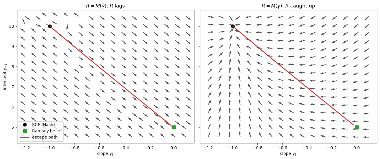
Fig. 104.4 Mean-dynamics drift with R lagging (left) and with R caught up (right), and the escape path#
In the left panel, with \(R\) at its Nash-era value, the arrows along the escape route sweep toward the Ramsey belief.
In the right panel, where \(R\) has caught up, they point back toward slope \(-\theta\) everywhere.
There the drift is \(T(\gamma) - \gamma\), whose slope component \(-\theta - \gamma_1\) is negative whenever \(\gamma_1 > -\theta\).
So the reinforcement is a property of the joint dynamics of \(\gamma\) and \(R\); it is the same lag that produced the dip in Fig. 104.2.
Along the escape path itself \(R\) moves only part of the way toward \(\bar M(\gamma)\), because the escape takes only a fraction of a unit of time; Exercise 104.2 measures the alignment with the path’s own \(R\).
The escape dynamics only need to start the departure; the mean dynamics finish the job.
This is the sense in which the mean dynamics trace a circuitous route: pushed off the equilibrium along the escape path, the system travels near Ramsey before \(R\) catches up, the residual short-run Phillips curve is rediscovered, and the mean dynamics eventually carry beliefs back to Nash.
104.9. The experimentation trap#
The escape has a compelling behavioural interpretation.
Within its approximating model, the government can only detect the natural-rate hypothesis if there is enough dispersion in inflation.
But inside a self-confirming equilibrium the government sets a constant systematic inflation rate, so it generates no such dispersion: it is caught in an experimentation trap.
Only an unusual run of shocks makes the government vary inflation enough to steepen its estimated Phillips curve; a steeper perceived curve leads it (through the best response) to cut inflation, which generates further influential observations that steepen the curve further.
As CWS note, overweighting recent observations helps this process along.
This self-reinforcing process halts when the perceived Phillips curve is vertical, and inflation is near Ramsey.
The system cannot stay there forever: in truth there is a short-run Phillips curve, which the government eventually rediscovers, rekindling the mean dynamics that carry it back to Nash.
104.10. Simulating escapes#
The large-deviation results describe the limit \(\varepsilon \to 0\).
To see what they imply at the gains this suite actually uses, we simulate the static model under the constant-gain recursion (104.4).
Every path starts at the self-confirming equilibrium, with \(R_0 = \bar M(\bar\gamma)\).
def simulate_path(model, ε, n_periods, seed=0):
    "One path of the static model under constant-gain RLS (en_rls), started at the SCE."
    rng = np.random.default_rng(seed)
    θ, u, σ1, σ2 = model.θ, model.u, model.σ1, model.σ2
    γ = model.γ_sce()
    R = model.M(γ)
    x_path, γ_path = np.empty(n_periods), np.empty((n_periods, 2))
    for n in range(n_periods):
        x = model.x(γ)
        w1, w2 = rng.standard_normal(2)
        π = x + σ2 * w2
        U = u - θ * σ2 * w2 + σ1 * w1
        Φ = np.array([π, 1.0])
        R = R + ε * (np.outer(Φ, Φ) - R)
        γ = γ + ε * np.linalg.solve(R, Φ * (U - Φ @ γ))
        x_path[n], γ_path[n] = x, γ
    return x_path, γ_path
We use \(\varepsilon = 0.02\), the gain of A government learning the Phillips curve; Adaptive Learning and Escape Dynamics uses \(0.025\), the book’s \(\lambda = .975\).
ε = 0.02
x_path, γ_path = simulate_path(model, ε, 4_000, seed=1)

fig, axes = plt.subplots(2, 1, figsize=(10, 6), sharex=True)
axes[0].plot(x_path, lw=0.8)
axes[0].axhline(model.θ * model.u, color='k', ls='--', lw=1, label='Nash')
axes[0].axhline(0, color='C2', ls=':', lw=1, label='Ramsey')
axes[0].set_ylabel('target inflation $x_n$')
axes[0].legend(loc='upper right')
axes[1].plot(γ_path[:, 0], lw=0.8, color='C1')
axes[1].axhline(-model.θ, color='k', ls='--', lw=1)
axes[1].set_ylabel(r'slope $\gamma_{1n}$')
axes[1].set_xlabel('period $n$')
plt.tight_layout()
plt.show()
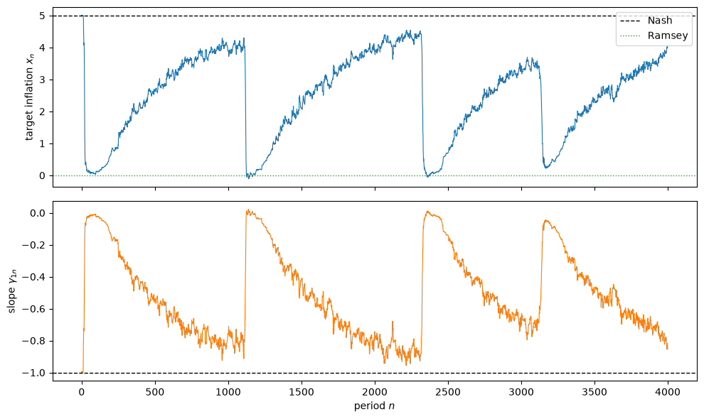
Fig. 104.5 A simulated path of the static model with gain 0.02#
Like the long simulation in A government learning the Phillips curve, the path is a recurrent sawtooth: abrupt escapes toward zero inflation, each followed by a slow climb back toward Nash, often interrupted by the next escape.
A longer run shows how little time the government spends near Nash.
x_long, _ = simulate_path(model, ε, 20_000, seed=2)
print(f"ε = {ε}, 20,000 periods:")
print(f"  share of periods with x > 4: {np.mean(x_long > 4):.2f}")
print(f"  share of periods with x < 2: {np.mean(x_long < 2):.2f}")
print(f"  mean target inflation:       {x_long.mean():.2f}   (Nash {model.θ * model.u:.0f})")
ε = 0.02, 20,000 periods:
  share of periods with x > 4: 0.10
  share of periods with x < 2: 0.34
  mean target inflation:       2.47   (Nash 5)
Target inflation is above 4 in only a small minority of periods.
To connect with the theorem, we measure the first exit time from the radius-5 circle, starting at the self-confirming equilibrium, for many independent paths.
def first_exits(model, ε, n_paths=400, radius=5.0, seed=0):
    """
    Simulate n_paths independent copies of (en_rls) from the SCE.  Return each
    path's first exit period from the circle of the given radius and its beliefs
    at exit (NaN if it has not exited after 100/ε periods).
    """
    rng = np.random.default_rng(seed)
    θ, u, σ1, σ2 = model.θ, model.u, model.σ1, model.σ2
    γ_bar = model.γ_sce()
    γ = np.tile(γ_bar, (n_paths, 1))
    R = np.tile(model.M(γ_bar), (n_paths, 1, 1))
    τ = np.full(n_paths, np.nan)
    γ_exit = np.full((n_paths, 2), np.nan)
    alive = np.ones(n_paths, dtype=bool)
    n = 0
    while alive.any() and n < 100 / ε:
        n += 1
        x = -γ[:, 1] * γ[:, 0] / (1 + γ[:, 0]**2)
        w1, w2 = rng.standard_normal((2, n_paths))
        π = x + σ2 * w2
        U = u - θ * σ2 * w2 + σ1 * w1
        Φ = np.stack([π, np.ones(n_paths)], axis=1)
        R += ε * (Φ[:, :, None] * Φ[:, None, :] - R)
        e = U - (Φ * γ).sum(axis=1)
        γ += ε * np.linalg.solve(R, (Φ * e[:, None])[:, :, None])[:, :, 0]
        out = alive & (np.linalg.norm(γ - γ_bar, axis=1) > radius)
        τ[out], γ_exit[out] = n, γ[out]
        alive &= ~out
    return τ, γ_exit


S_bar = 4.987e-4        # CWS Table 1: static model, normal shocks, radius 5

print(f"{'ε':>6s} {'mean':>7s} {'median':>7s} {'ε·mean':>7s} {'exp(S̄/ε)':>9s} "
      f"{'x at exit < 1':>13s} {'not exited':>10s}")
for ε in [0.1, 0.05, 0.03, 0.02, 0.01, 0.005]:
    τ, γ_exit = first_exits(model, ε)
    done = ~np.isnan(τ)
    x_exit = -γ_exit[done, 1] * γ_exit[done, 0] / (1 + γ_exit[done, 0]**2)
    print(f"{ε:6.3f} {np.mean(τ[done]):7.1f} {np.median(τ[done]):7.0f} "
          f"{ε * np.mean(τ[done]):7.2f} {np.exp(S_bar / ε):9.3f} "
          f"{np.mean(x_exit < 1):13.2f} {np.sum(~done):10d}")
print(f"\nexp(S̄/ε) at ε = 0.0002: {np.exp(S_bar / 0.0002):.1f}")
     ε    mean  median  ε·mean exp(S̄/ε) x at exit < 1 not exited
 0.100    15.8      11    1.58     1.005          1.00          0
 0.050    27.6      22    1.38     1.010          1.00          0
 0.030    46.1      36    1.38     1.017          1.00          0
 0.020    77.1      59    1.54     1.025          1.00          0
 0.010   173.6     135    1.74     1.051          1.00          0
 0.005   405.5     329    2.03     1.105          1.00          0

exp(S̄/ε) at ε = 0.0002: 12.1
Mean first exit times run from about 16 periods at \(\varepsilon = 0.1\) to about 400 at \(\varepsilon = 0.005\).
At \(\varepsilon = 0.01\) and \(0.005\) they are close to the 165.7 and 409.6 periods that Sargent and Williams [2005] (Table 1) report for constant-gain least squares.
Every path exits on the Ramsey side, near the exit point of the escape path.
The product \(\varepsilon \times\) mean stays between about 1.4 and 2, so mean exit times scale roughly like \(1/\varepsilon\).
The factor \(e^{\bar S/\varepsilon}\), by contrast, never exceeds 1.11 in the table.
At these gains the large-deviation factor plays almost no role; exit times are set by the constant \(S_0\), that is, by how long beliefs take to wander off the equilibrium and travel the route.
At the gains this suite uses, escapes are frequent, not rare.
Starting from the self-confirming equilibrium, a government with gain \(\varepsilon\) escapes on average after roughly \(1.5/\varepsilon\) to \(2/\varepsilon\) periods, and between escapes it seldom gets all the way back to Nash.
Rarity is a small-gain statement.
Only for gains of the order of \(\bar S\) itself does the exponential factor bite: at \(\varepsilon = 0.0002\), five times smaller than the smallest gain in Table 1 of Sargent and Williams [2005], \(e^{\bar S/\varepsilon} \approx 12\).
The simulated exit times also bear out CWS’s footnote 14.
Measured in units of \(t = n\varepsilon\), they are several times the \(0.34\) that the changed-measure path takes; Exercise 104.5 compares the two in detail.
104.11. Escape frequency and model richness#
The minimized action \(\bar S\) sets the exponential rate at which escape times grow as the gain shrinks.
A striking finding of CWS is that escapes are more frequent when the government’s model is richer.
CWS’s Table 1 gives the dynamic model of Adaptive Learning and Escape Dynamics, with lagged unemployment and inflation, a rate \(\bar S \approx 9.7 \times 10^{-6}\), about fifty times smaller than the static model’s \(5.0 \times 10^{-4}\), even though the two share the same self-confirming equilibrium.
That dynamic-model number needs a caveat: it was computed with the 2001 shortcut that Williams [2019] corrected, which matters for dynamic models.
The comparison does not rest on that number alone, though.
In CWS’s simulations (their Figure 5), mean escape times are shorter in the dynamic model at every gain, and Exercise 104.6 finds the same for median first-escape times.
A richer model lets the government detect the subtler distributed-lag (“induction-hypothesis”) version of the natural-rate hypothesis, so it escapes toward Ramsey more readily.
Note
The escape dynamics inherit the same “near determinism” that makes the mean dynamics useful: for small gains, simulated escapes cluster around the deterministic escape route, in the dynamic model (CWS, Figure 6) and in the static model (Exercise 104.5; CWS, Figure 7).
The next lecture, Priors, Escapes, and Learning Cycles, shows that the government’s prior about how its coefficients drift reshapes both dynamics, and can even make the escape a deterministic cycle.
104.12. Escaping volatile inflation#
The escape delivers a fall in the level of inflation.
Ellison and Yates [2007] extend the model to explain a second post-war fact: inflation volatility rose and fell together with the level.
Their device is to give the government a reason to stabilize.
Following Phelps and Taylor [1977], they add an unemployment shock \(W_3\) that the government, but not the price-setting private sector, can react to.
Now a government that believes in an exploitable Phillips curve is tempted to lean against \(W_3\) by varying inflation, so the perceived effectiveness of policy, \(|\gamma_1|\), drives the volatility of inflation as well as its level.
In their model the expected inflation volatility a private agent faces is
At the self-confirming equilibrium \(\gamma_1 = -\theta\), the government believes policy is effective and leans against \(W_3\) aggressively, so inflation is volatile.
Along an escape, \(\gamma_1 \to 0\): the government stops believing it can exploit the Phillips curve, abandons stabilization, and the volatility term collapses to the control error \(\sigma_2\).
As an approximation, we apply (104.11) to the belief path computed above for \(\sigma_3 = 0\).
In Ellison and Yates’s model a positive \(\sigma_3\) also changes the escape itself, as we discuss below, but the approximation shows the level and volatility of inflation escaping in tandem.
σ3 = 0.9                                   # size of the stabilizable shock
infl_vol = np.sqrt(model.σ2**2 + (slope / (1 + slope**2))**2 * σ3**2)

fig, axes = plt.subplots(1, 2, figsize=(12, 4.5))
axes[0].plot(esc.t, infl)
axes[0].axhline(model.θ * model.u, color='k', ls='--', lw=1, label='Nash')
axes[0].axhline(0, color='C2', ls=':', lw=1, label='Ramsey')
axes[0].set_xlabel('time $t = n\\varepsilon$'); axes[0].set_ylabel('inflation level')
axes[0].set_title('level escapes'); axes[0].legend()

axes[1].plot(esc.t, infl_vol, 'C1')
axes[1].axhline(model.σ2, color='k', ls='--', lw=1, label=r'control error $\sigma_2$')
axes[1].set_xlabel('time $t = n\\varepsilon$'); axes[1].set_ylabel('inflation volatility')
axes[1].set_title('volatility escapes too'); axes[1].legend()

plt.tight_layout()
plt.show()
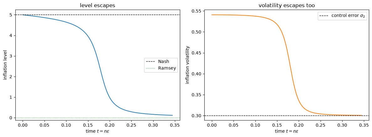
Fig. 104.6 The level and volatility of inflation escape in tandem#
Both fall as beliefs escape, because both spring from the same source: the government’s belief in an exploitable tradeoff.
Ellison and Yates [2007] draw a further, subtler lesson about the timing of escapes.
A larger stabilizable shock \(\sigma_3\) makes an escape harder to trigger: to create the illusion that inflation moves while unemployment stays put, an unusual sequence of shocks must now offset not only the control errors but also the government’s own stabilizing reaction to \(W_3\).
The more shocks the government can offset, the more complex the escape-triggering sequence, and the longer the wait.
Ellison and Yates conclude that an escape to low inflation is more likely in a period with relatively few shocks that policy can offset.
It is tempting, and it is our extrapolation rather than theirs, to read the calm of the mid-1980s as such a period, and to link it to the disinflation.
The timing does not fit easily.
In the estimates of Drifts and Volatilities, core inflation fell in 1980–82, while most of the decline in the variance of shocks came in the mid-1980s.
The disinflation came first, during a period of unusually large shocks.
That lecture builds a statistical model with room for both shrinking shocks and shifting dynamics and lets the data apportion them.
Before turning to data, Priors, Escapes, and Learning Cycles returns to the static model and asks how the government’s prior about drifting coefficients changes everything above.
104.13. Exercises#
Exercise 104.1
At the self-confirming equilibrium the moment matrix is \(\bar R = \bar M(\bar\gamma)\), with \(\det \bar R = \sigma_2^2\).
Show that the escape velocity at the self-confirming equilibrium is \(\bar R^{-1}(\sigma_1\sigma_2, 0)^\top = (\sigma_1/\sigma_2)(1, -\bar x)^\top\), where \(\bar x = \theta u\). So with \(\sigma_1 = \sigma_2\) it does not depend on the size of the shocks.
Integrate the escape ODE (104.9) for \(\sigma_1 = \sigma_2 = \sigma \in \{0.1, 0.2, 0.3, 0.4, 0.5\}\) and report the exit time from the radius-5 circle.
Exit times nonetheless rise with \(\sigma\). Explain why. Hint: write \(\bar M(\gamma) = \bar R + \Delta(\gamma)\) and look at how \(\Delta\) and \(\bar R^{-1}\) depend on \(\sigma_2\).
Now vary one shock at a time: \(\sigma_2 \in \{0.2, 0.3, 0.45\}\) with \(\sigma_1 = 0.3\), and \(\sigma_1 \in \{0.2, 0.3, 0.45\}\) with \(\sigma_2 = 0.3\).
Solution
For part 1, \(\bar R = \begin{bmatrix} \bar x^2 + \sigma_2^2 & \bar x \\ \bar x & 1 \end{bmatrix}\) has determinant \(\sigma_2^2\) and inverse \(\sigma_2^{-2}\begin{bmatrix} 1 & -\bar x \\ -\bar x & \bar x^2 + \sigma_2^2 \end{bmatrix}\), so \(\bar R^{-1}(\sigma_1\sigma_2, 0)^\top = (\sigma_1/\sigma_2)(1, -\bar x)^\top\).
For parts 2 and 4, we integrate the escape ODE for each pair of shock sizes.
def exit_time(σ1, σ2):
    m = EscapeModel(θ=1.0, u=5.0, σ1=σ1, σ2=σ2)
    γ0 = m.γ_sce()

    def leave(t, z):
        return 5.0 - np.linalg.norm(z[:2] - γ0)
    leave.terminal = True
    leave.direction = -1

    v0 = np.linalg.solve(m.M(γ0), np.array([σ1 * σ2, 0.0]))
    s = solve_ivp(lambda t, z: escape_ode(t, z, m), [0, 500],
                  np.concatenate([γ0, m.M(γ0).ravel()]),
                  events=leave, max_step=0.02, rtol=1e-9, atol=1e-11)
    return v0, s.t[-1]

for σ in [0.1, 0.2, 0.3, 0.4, 0.5]:
    v0, T = exit_time(σ, σ)
    print(f"σ1 = σ2 = {σ}: velocity at SCE = {v0.round(3)}, exit time = {T:.3f}")
print()
for σ2 in [0.2, 0.3, 0.45]:
    print(f"σ1 = 0.3, σ2 = {σ2}: exit time = {exit_time(0.3, σ2)[1]:.3f}")
for σ1 in [0.2, 0.3, 0.45]:
    print(f"σ1 = {σ1}, σ2 = 0.3: exit time = {exit_time(σ1, 0.3)[1]:.3f}")
σ1 = σ2 = 0.1: velocity at SCE = [ 1. -5.], exit time = 0.083
σ1 = σ2 = 0.2: velocity at SCE = [ 1. -5.], exit time = 0.201
σ1 = σ2 = 0.3: velocity at SCE = [ 1. -5.], exit time = 0.344
σ1 = σ2 = 0.4: velocity at SCE = [ 1. -5.], exit time = 0.503
σ1 = σ2 = 0.5: velocity at SCE = [ 1. -5.], exit time = 0.671

σ1 = 0.3, σ2 = 0.2: exit time = 0.171
σ1 = 0.3, σ2 = 0.3: exit time = 0.344
σ1 = 0.3, σ2 = 0.45: exit time = 0.740
σ1 = 0.2, σ2 = 0.3: exit time = 0.411
σ1 = 0.3, σ2 = 0.3: exit time = 0.344
σ1 = 0.45, σ2 = 0.3: exit time = 0.285
With \(\sigma_1 = \sigma_2\) the starting velocity is the same for every \(\sigma\), yet the exit time rises steadily with \(\sigma\).
The speed comes from the \(R\)-lag amplification of Mean dynamics reinforce the escape.
During the escape \(R\) stays near \(\bar R\), so the mean drift is \(\bar R^{-1}\bar M(\gamma)(T(\gamma) - \gamma) = (T(\gamma) - \gamma) + \bar R^{-1}\Delta(\gamma)(T(\gamma) - \gamma)\).
Here \(\Delta(\gamma) = \begin{bmatrix} x^2 - \bar x^2 & x - \bar x \\ x - \bar x & 0 \end{bmatrix}\) depends only on how far inflation has moved, not on \(\sigma_2\), while \(\bar R^{-1}\) is of order \(1/\sigma_2^2\).
So the smaller the control error, the more strongly the lagging moment matrix amplifies any move away from Nash, and the faster beliefs travel the route.
That is why \(\sigma_2\) matters so much in part 4, while a larger \(\sigma_1\) speeds the escape only through the initial push \(\sigma_1/\sigma_2\).
None of this concerns the frequency of escapes, which Simulating escapes measures; a noisier economy travels the deterministic route more slowly once an escape is under way.
Exercise 104.2
Make the reinforcement in the vector-field plot quantitative.
At several points along the escape path, evaluate the mean-dynamics drift \(R^{-1}\bar g(\gamma)\), with the path’s own \(R\), and measure its cosine alignment with the direction from the current beliefs toward the Ramsey belief \((0, u)\).
A cosine near \(+1\) means the mean dynamics are pushing beliefs toward Ramsey, reinforcing the escape.
Solution
We evaluate the drift at five points along the escape path.
γ_ramsey = np.array([0.0, model.u])            # Belief 2

def cosine_toward_ramsey(γ, R):
    drift = np.linalg.solve(R, model.g_bar(γ))
    to_ramsey = γ_ramsey - γ
    denom = np.linalg.norm(drift) * np.linalg.norm(to_ramsey)
    return np.nan if denom < 1e-9 else drift @ to_ramsey / denom

for frac in [0.0, 0.25, 0.5, 0.75, 0.95]:
    k = min(int(frac * len(esc.t)), len(esc.t) - 1)
    γ, R = esc.y[:2, k], esc.y[2:, k].reshape(2, 2)
    print(f"frac {frac:.2f}:  γ = ({γ[0]:+.2f}, {γ[1]:.1f}),  "
          f"cos(drift, →Ramsey) = {cosine_toward_ramsey(γ, R):+.2f},  "
          f"with R = M(γ): {cosine_toward_ramsey(γ, model.M(γ)):+.2f}")
frac 0.00:  γ = (-1.00, 10.0),  cos(drift, →Ramsey) = +nan,  with R = M(γ): +nan
frac 0.25:  γ = (-0.65, 8.2),  cos(drift, →Ramsey) = +1.00,  with R = M(γ): -0.93
frac 0.50:  γ = (-0.23, 6.1),  cos(drift, →Ramsey) = +1.00,  with R = M(γ): -0.47
frac 0.75:  γ = (-0.07, 5.3),  cos(drift, →Ramsey) = +1.00,  with R = M(γ): -0.25
frac 0.95:  γ = (-0.03, 5.1),  cos(drift, →Ramsey) = +1.00,  with R = M(γ): -0.25
Right at the self-confirming equilibrium the drift vanishes (the cosine is undefined), so the mean dynamics neither help nor hinder.
But once beliefs have moved even slightly along the escape route, the mean-dynamics drift points almost exactly toward the Ramsey belief (cosine \(\approx +1\)): the mean dynamics reinforce the escape all the way to Ramsey.
The last column replaces the path’s \(R\) by \(\bar M(\gamma)\), and the cosine turns negative: the reinforcement comes from \(R\) lagging behind.
The opposition that CWS emphasize is confined to a tiny neighbourhood of the equilibrium; the escape dynamics only need to nudge beliefs out of it, after which the mean dynamics finish the job.
Exercise 104.3
Look more closely at the race of four ODEs.
Plot the four conditional paths
racein the \((\gamma_1, \gamma_{-1})\) plane, together with the radius-5 circle, and plot inflation along each.CWS give the rest points of the conditional ODEs for pairs 3 and 4 as \((-\theta,\ (u \pm \sigma_1)(1+\theta^2))\), both well inside the circle. Pair 3 settles there. Why does pair 4 escape instead?
Rerun the race with \(R\) held equal to \(\bar M(\gamma)\), as if the moment matrix adjusted instantly. Which pair wins now, and where does it exit?
Solution
We first plot the four paths computed in the text.
fig, axes = plt.subplots(1, 2, figsize=(13, 5))
φ = np.linspace(0, 2 * np.pi, 200)
axes[0].plot(γ_sce[0] + 5 * np.cos(φ), γ_sce[1] + 5 * np.sin(φ), 'k:', lw=1)
for name, s in race.items():
    axes[0].plot(s.y[0], s.y[1], label=name)
    axes[1].plot(s.t, -s.y[1] * s.y[0] / (1 + s.y[0]**2), label=name)
axes[0].plot(*γ_sce, 'ko')
axes[0].set_xlabel(r'slope $\gamma_1$')
axes[0].set_ylabel(r'intercept $\gamma_{-1}$')
axes[1].set_xscale('log')
axes[1].set_xlabel('time $t$ (log scale)')
axes[1].set_ylabel('inflation $x$')
axes[0].legend()
plt.tight_layout()
plt.show()
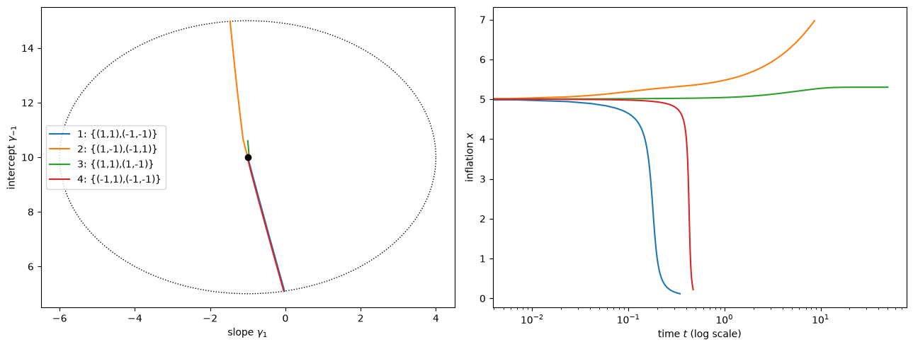
Next we rerun the race with \(R = \bar M(\gamma)\) imposed, which reduces each conditional ODE to \(\dot\gamma = T(\gamma) - \gamma + \bar M(\gamma)^{-1} f_j(\gamma)\).
def cond_ode_no_lag(t, γ, model, f):
    return np.linalg.solve(model.M(γ), model.g_bar(γ) + f(γ, model))

def left_circle_γ(t, γ, *args):
    return 5.0 - np.linalg.norm(γ - γ_sce)
left_circle_γ.terminal = True
left_circle_γ.direction = -1

for name, f in pairs.items():
    s = solve_ivp(cond_ode_no_lag, [0, 50], γ_sce, args=(model, f), events=left_circle_γ,
                  max_step=0.02, rtol=1e-9, atol=1e-11)
    γ_end = s.y[:, -1]
    status = f"exits at t = {s.t[-1]:.3f}" if s.status == 1 else "never exits"
    print(f"{name:22s} {status:22s} γ_end = ({γ_end[0]:+.3f}, {γ_end[1]:.2f}), "
          f"x = {model.x(γ_end):.2f}")
1: {(1,1),(-1,-1)}     exits at t = 3.941     γ_end = (-0.019, 5.10), x = 0.10
2: {(1,-1),(-1,1)}     exits at t = 1.194     γ_end = (-1.697, 14.95), x = 6.54
3: {(1,1),(1,-1)}      never exits            γ_end = (-1.000, 10.60), x = 5.30
4: {(-1,1),(-1,-1)}    never exits            γ_end = (-1.000, 9.40), x = 4.70
With \(R = \bar M(\gamma)\) the rest point of each conditional ODE is a fixed point of a shifted \(T\)-map.
For pair 4 it is \((-\theta, (u - \sigma_1)(1+\theta^2))\); the Jacobian of the drift there again has eigenvalues \(-1\) and \(-1/(1+\theta^2)\), so the path converges to it.
With the true, lagging \(R\), the same forcing first lowers the intercept and inflation a little; the lagging moment matrix then amplifies the move into a full escape to Ramsey.
Without the lag, the race changes completely.
Pair 1 still heads for Ramsey but only drifts there slowly, while pair 2 now exits first, toward higher inflation.
So the \(R\) lag decides both the direction and the speed of the escape: it is what makes the Ramsey-ward route the most likely one.
Exercise 104.4
The theorem says \(\varepsilon \log \mathbb{E}\,\tau^\varepsilon \to \bar S\), where \(\tau^\varepsilon = n\varepsilon\) is the exit time on the ODE time scale; equivalently \(\log \mathbb{E}\,\tau^\varepsilon \approx S_0 + \bar S/\varepsilon\).
Use
first_exitsto compute the mean exit period for \(\varepsilon \in \{0.1, 0.05, 0.02, 0.01, 0.005, 0.0025, 0.001\}\).Plot \(\log(\varepsilon \times \text{mean exit period})\) against \(1/\varepsilon\), and compare the slope with CWS’s \(\bar S\).
Compare the mean exit periods with Sargent and Williams [2005] (Table 1), who report 20.6, 165.7, 409.6, 2414.8 and 4486.7 periods at \(\varepsilon = 0.05, 0.01, 0.005, 0.002, 0.001\).
Solution
We compute the mean exit period on a finer grid of small gains.
gains = np.array([0.1, 0.05, 0.02, 0.01, 0.005, 0.0025, 0.001])
mean_exit = np.array([np.nanmean(first_exits(model, ε, seed=1)[0]) for ε in gains])
log_scaled = np.log(gains * mean_exit)

for ε, m, l in zip(gains, mean_exit, log_scaled):
    print(f"ε = {ε:6.4f}: mean exit period = {m:7.0f},  ε·mean = {ε * m:5.2f}")
local_slope = np.diff(log_scaled) / np.diff(1 / gains)
print("\nlocal slopes of log(ε·mean) in 1/ε:", local_slope.round(5))
print(f"CWS S̄ = {S_bar:.5f}")

fig, ax = plt.subplots(figsize=(7, 4.5))
ax.plot(1 / gains, log_scaled, 'o-', label='simulation')
ax.plot(1 / gains, log_scaled[-1] + S_bar * (1 / gains - 1 / gains[-1]), 'k--',
        label=r'slope $\bar S$ (CWS), through last point')
ax.set_xlabel(r'$1/\varepsilon$')
ax.set_ylabel(r'$\log(\varepsilon \times$ mean exit period$)$')
ax.legend()
plt.show()
ε = 0.1000: mean exit period =      15,  ε·mean =  1.47
ε = 0.0500: mean exit period =      28,  ε·mean =  1.39
ε = 0.0200: mean exit period =      72,  ε·mean =  1.43
ε = 0.0100: mean exit period =     164,  ε·mean =  1.64
ε = 0.0050: mean exit period =     426,  ε·mean =  2.13
ε = 0.0025: mean exit period =    1114,  ε·mean =  2.79
ε = 0.0010: mean exit period =    4629,  ε·mean =  4.63

local slopes of log(ε·mean) in 1/ε: [-0.00525  0.001    0.00272  0.00259  0.00135  0.00085]
CWS S̄ = 0.00050
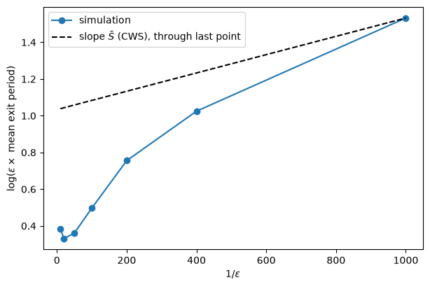
The scaled mean \(\varepsilon \times\) mean stays between about 1.4 and 4.6 over a hundredfold range of gains.
Over that range \(\bar S/\varepsilon\) rises only from 0.005 to 0.5, so the level of \(\log \mathbb{E}\,\tau^\varepsilon\) is dominated by the constant \(S_0\).
At large gains the curve even slopes down, and only at the smallest gains does its slope approach the order of magnitude of \(\bar S\): the asymptotic regime of the theorem lies at gains far smaller than those this suite uses.
The simulated means agree closely with SW’s at \(\varepsilon = 0.01\), \(0.005\) and \(0.001\).
Exercise 104.5
CWS’s Figure 7 compares simulated escapes with the dominant and changed-measure paths.
Simulate 50 paths at \(\varepsilon = 0.005\) from the self-confirming equilibrium, recording beliefs until each first leaves the radius-5 circle.
Plot the slope and intercept of each path against \(\log n\), together with the changed-measure path at \(n = t/\varepsilon\).
Compare the exit points, the total time to exit, and the duration of the final run, measured from the last period in which the slope is below \(-0.9\).
Solution
We record the full belief history of each path until it exits.
def escape_histories(model, ε, n_paths=50, n_max=10_000, radius=5.0, seed=0):
    rng = np.random.default_rng(seed)
    θ, u, σ1, σ2 = model.θ, model.u, model.σ1, model.σ2
    γ_bar = model.γ_sce()
    γ = np.tile(γ_bar, (n_paths, 1))
    R = np.tile(model.M(γ_bar), (n_paths, 1, 1))
    hist = np.full((n_max + 1, n_paths, 2), np.nan)
    hist[0] = γ
    τ = np.zeros(n_paths, dtype=int)
    alive = np.ones(n_paths, dtype=bool)
    for n in range(1, n_max + 1):
        x = -γ[:, 1] * γ[:, 0] / (1 + γ[:, 0]**2)
        w1, w2 = rng.standard_normal((2, n_paths))
        π = x + σ2 * w2
        U = u - θ * σ2 * w2 + σ1 * w1
        Φ = np.stack([π, np.ones(n_paths)], axis=1)
        R += ε * (Φ[:, :, None] * Φ[:, None, :] - R)
        e = U - (Φ * γ).sum(axis=1)
        γ += ε * np.linalg.solve(R, (Φ * e[:, None])[:, :, None])[:, :, 0]
        hist[n, alive] = γ[alive]
        out = alive & (np.linalg.norm(γ - γ_bar, axis=1) > radius)
        τ[out] = n
        alive &= ~out
        if not alive.any():
            break
    return hist[:n + 1], τ

ε = 0.005
hist, τ = escape_histories(model, ε, seed=3)
print(f"all exited: {np.all(τ > 0)}")
print(f"simulated exit periods: min {τ.min()}, median {np.median(τ):.0f}, max {τ.max()}")
print(f"changed-measure path:   exits at n = t/ε = {esc.t[-1] / ε:.0f}")

γ_end = hist[τ, np.arange(len(τ))]
print(f"exit slope: simulated mean {γ_end[:, 0].mean():+.3f}, "
      f"changed-measure {slope[-1]:+.3f}")

final_run = np.array([(τ[i] - np.where(hist[:τ[i] + 1, i, 0] < -0.9)[0].max()) * ε
                      for i in range(len(τ))])
k_cm = np.where(slope < -0.9)[0].max()
print(f"final run (in t = nε): simulated median {np.median(final_run):.2f}, "
      f"changed-measure {esc.t[-1] - esc.t[k_cm]:.2f}")
all exited: True
simulated exit periods: min 124, median 366, max 1072
changed-measure path:   exits at n = t/ε = 69
exit slope: simulated mean -0.024, changed-measure -0.023
final run (in t = nε): simulated median 0.35, changed-measure 0.26
Next we plot the paths on CWS’s log time scale.
fig, ax = plt.subplots(figsize=(9, 5))
for i in range(len(τ)):
    n_i = np.arange(1, τ[i] + 1)
    ax.plot(np.log(n_i), hist[1:τ[i] + 1, i, 1], color='C0', lw=0.4, alpha=0.5)
    ax.plot(np.log(n_i), hist[1:τ[i] + 1, i, 0], color='C1', lw=0.4, alpha=0.5)
n_cm = esc.t[1:] / ε
ax.plot(np.log(n_cm), intercept[1:], 'k--', lw=2, label='changed measure: intercept')
ax.plot(np.log(n_cm), slope[1:], 'k-.', lw=2, label='changed measure: slope')
ax.set_xlabel(r'$\log n$')
ax.set_ylabel('coefficient')
ax.set_title(f'50 simulated escapes (ε = {ε}) and the changed-measure path')
ax.legend()
plt.show()
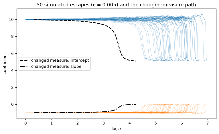
The simulated escapes leave the circle at almost exactly the changed-measure path’s exit point, as Theorem 5.3 predicts for the dominant path.
But the changed-measure path exits before even the fastest simulated escape, as CWS found.
Most of the difference is waiting time: a simulated path spends a long spell near the self-confirming equilibrium before its final run.
Once that run is under way, it takes a time of the same order as the changed-measure path.
Exercise 104.6
CWS find escapes more frequent in their dynamic model than in the static one.
Check this by simulation.
In the dynamic model of Adaptive Learning and Escape Dynamics (which writes \(y\) for inflation), the government regresses \(U_n\) on \((\pi_n, U_{n-1}, U_{n-2}, \pi_{n-1}, \pi_{n-2}, 1)\) and sets inflation by solving the discounted Phelps problem with \(\delta = 0.98\).
Simulate the dynamic model with the recursion (104.4), now with six regressors, starting at its self-confirming equilibrium with \(R_0\) equal to the self-confirming moment matrix.
Define the first escape as the first period in which the 20-period average of inflation falls below 1.
Report the median first escape over many paths for both models, for \(\varepsilon \in \{0.002, 0.005, 0.01, 0.02\}\).
Solution
The government’s decision rule uses the same Phelps solver as Adaptive Learning and Escape Dynamics.
The state is \((U_{n-1}, U_{n-2}, \pi_{n-1}, \pi_{n-2}, 1)\), and the cross term of the discounted Riccati equation enters unscaled.
def phelps_rule(γ, δ=0.98):
    "Rule π̂_n = h·(U_{n-1}, U_{n-2}, π_{n-1}, π_{n-2}, 1) for beliefs γ."
    γ0, c = γ[0], γ[1:]
    A, B = np.zeros((5, 5)), np.zeros((5, 1))
    A[0, :], B[0, 0] = c, γ0            # U_n
    A[1, 0] = 1.0                        # U_{n-1}
    B[2, 0] = 1.0                        # π_n
    A[3, 2] = 1.0                        # π_{n-1}
    A[4, 4] = 1.0                        # constant
    Q_x, Q_u, N = np.outer(c, c), np.array([[γ0**2 + 1.0]]), (γ0 * c).reshape(1, -1)
    Ad, Bd = np.sqrt(δ) * A, np.sqrt(δ) * B
    P = solve_discrete_are(Ad, Bd, Q_x, Q_u, s=N.T)
    F = np.linalg.solve(Q_u + Bd.T @ P @ Bd, Bd.T @ P @ Ad + N)
    return -F.ravel()


def dynamic_sce(model):
    "SCE beliefs and moments of (π_n, U_{n-1}, U_{n-2}, π_{n-1}, π_{n-2}, 1)."
    θ, u, σ1, σ2 = model.θ, model.u, model.σ1, model.σ2
    γ = np.array([-θ, 0, 0, 0, 0, (1 + θ**2) * u])
    mean = np.array([θ * u, u, u, θ * u, θ * u, 1.0])
    lag = [0, 1, 2, 1, 2, None]                       # date of each regressor
    var = {('π', 'π'): σ2**2, ('U', 'U'): θ**2 * σ2**2 + σ1**2,
           ('π', 'U'): -θ * σ2**2, ('U', 'π'): -θ * σ2**2}
    kind = ['π', 'U', 'U', 'π', 'π', 'c']
    M = np.outer(mean, mean)
    for i in range(6):
        for j in range(6):
            if lag[i] is not None and lag[i] == lag[j]:
                M[i, j] += var[(kind[i], kind[j])]
    return γ, M


def first_escape_dynamic(model, ε, seed, n_max=10_000, window=20):
    rng = np.random.default_rng(seed)
    θ, u, σ1, σ2 = model.θ, model.u, model.σ1, model.σ2
    γ, R = dynamic_sce(model)
    U1 = U2 = u
    π1 = π2 = θ * u
    recent = np.full(window, θ * u)
    for n in range(n_max):
        π_hat = phelps_rule(γ) @ np.array([U1, U2, π1, π2, 1.0])
        w1, w2 = rng.standard_normal(2)
        π = π_hat + σ2 * w2
        U = u - θ * σ2 * w2 + σ1 * w1
        Φ = np.array([π, U1, U2, π1, π2, 1.0])
        R = R + ε * (np.outer(Φ, Φ) - R)
        γ = γ + ε * np.linalg.solve(R, Φ * (U - Φ @ γ))
        U2, U1, π2, π1 = U1, U, π1, π
        recent[n % window] = π
        if n >= window and recent.mean() < 1:
            return n + 1
    return np.nan


def first_escape_static(model, ε, n_paths=200, n_max=20_000, window=20, seed=0):
    rng = np.random.default_rng(seed)
    θ, u, σ1, σ2 = model.θ, model.u, model.σ1, model.σ2
    γ = np.tile(model.γ_sce(), (n_paths, 1))
    R = np.tile(model.M(model.γ_sce()), (n_paths, 1, 1))
    recent = np.full((n_paths, window), θ * u)
    τ = np.full(n_paths, np.nan)
    alive = np.ones(n_paths, dtype=bool)
    for n in range(n_max):
        x = -γ[:, 1] * γ[:, 0] / (1 + γ[:, 0]**2)
        w1, w2 = rng.standard_normal((2, n_paths))
        π = x + σ2 * w2
        U = u - θ * σ2 * w2 + σ1 * w1
        Φ = np.stack([π, np.ones(n_paths)], axis=1)
        R += ε * (Φ[:, :, None] * Φ[:, None, :] - R)
        e = U - (Φ * γ).sum(axis=1)
        γ += ε * np.linalg.solve(R, (Φ * e[:, None])[:, :, None])[:, :, 0]
        recent[:, n % window] = π
        hit = alive & (n >= window) & (recent.mean(axis=1) < 1)
        τ[hit] = n + 1
        alive &= ~hit
        if not alive.any():
            break
    return τ


print("check: dynamic rule at the SCE =", phelps_rule(dynamic_sce(model)[0]).round(4))
check: dynamic rule at the SCE = [-0. -0. -0. -0. 5.]
Now we compare median first escapes.
print(f"{'ε':>6s} {'static median':>14s} {'dynamic median':>15s}")
for ε in [0.002, 0.005, 0.01, 0.02]:
    τ_s = first_escape_static(model, ε)
    τ_d = np.array([first_escape_dynamic(model, ε, seed) for seed in range(24)])
    print(f"{ε:6.3f} {np.nanmedian(τ_s):14.0f} {np.nanmedian(τ_d):15.0f}"
          f"   (not escaped: {np.isnan(τ_s).sum()}/{len(τ_s)}, {np.isnan(τ_d).sum()}/{len(τ_d)})")
     ε  static median  dynamic median
 0.002            948             200   (not escaped: 0/200, 0/24)
 0.005            286             102   (not escaped: 0/200, 0/24)
 0.010            121              52   (not escaped: 0/200, 0/24)
 0.020             62              32   (not escaped: 0/200, 0/24)
At every gain the dynamic model escapes sooner, and the gap widens as the gain falls, as CWS’s smaller \(\bar S\) for the dynamic model suggests.
The government with lags can find the induction hypothesis while keeping a short-run Phillips curve, so it needs a less unusual run of shocks to begin the escape.
The comparison holds even though the two models share the same self-confirming equilibrium.