94. Networks, Genetic Algorithms, and Classifier Systems#
94.1. Overview#
The lectures so far gave adaptive agents a fairly econometric brain.
In Adaptive Agents in an Overlapping Generations Monetary Economy they ran stochastic approximation and recursive least squares, in Learning, Approximation, and Equilibrium Computation they fitted conditional expectations, and in Exchange Rate Indeterminacy, Learning, and Experiments they took Newton steps against realized utility.
Each of those learners was told what to estimate (a saving rate, a conditional expectation, a portfolio) and updated its estimate by a recursion of the kind described in One recursion, many learners.
Exchange Rate Indeterminacy, Learning, and Experiments also gave a first look at a learner of another kind: Arifovic’s genetic-algorithm economy (A genetic algorithm economy), whose exchange rate never settles down.
This lecture sets out that algorithm and its relatives in general.
They make up the toolbox that Sargent [1993] draws from John Holland’s work on adaptive systems [Holland, 1975, Holland et al., 1986] and from the connectionist literature on neural networks.
Sargent’s framing is that the bounded-rationality program asks us to populate models with agents who “behave like econometricians,” and that the artificial-intelligence literature is a catalogue of candidate brains for them:
It is from the store of methods built up in these literatures that we shall select the ‘brains’ to give our boundedly rational agents.
We tour four of them:
the perceptron, the simplest neural network, which turns out to be a linear discriminant function, a direct link to the “agents as econometricians” reading;
the Hopfield network, an associative memory that recovers stored patterns from corrupted inputs by rolling downhill on an energy function;
the genetic algorithm, Holland’s population-based search, which we set loose on Axelrod’s iterated prisoner’s dilemma;
the classifier system, Holland’s “brain as a competitive economy” of if-then rules, whose simplest instance, a two-armed bandit, already exposes a subtle limitation, and whose bucket brigade passes credit back along chains of decisions.
The first two are bridges from what came before.
The perceptron is a parametric rule that an econometrician recognizes on sight, and the Hopfield network is a memory rather than a rule.
The last two do something new: instead of tuning the coefficients of a fixed rule, they discover rules, searching a large space of possibilities with experience as the only guide.
We close with evolutionary programming: the idea that a population of adaptive agents, plodding toward an equilibrium, can be used to compute equilibria that we cannot solve for directly.
That is the idea Money as a Medium of Exchange among Artificially Intelligent Agents carries out in full, and this lecture builds the machinery it uses.
Let’s start with some imports.
import numpy as np
import matplotlib.pyplot as plt
94.2. The perceptron: an agent as a discriminant function#
The simplest neural network is a single perceptron: \(k\) inputs \(x_i\), weights \(w_i\), and one output
where \(S\) is a “squasher” mapping \(\mathbb{R}\) onto \([0, 1]\): a step function, or the sigmoid \(S(z) = 1/(1 + e^{-z})\), or any cumulative distribution function.
For fixed weights the perceptron is a classifier: it fires (\(y = 1\)) when \(w^\top x > 0\) and stays quiet otherwise, so the boundary \(w^\top x = 0\) is a hyperplane separating two classes.
Training the perceptron, that is, choosing \(w\) to minimize \(\sum_t (y_t - S(w^\top x_t))^2\), is a nonlinear least squares problem, solved by the stochastic-gradient recursion
where \(\nabla S(w, x)\) is the gradient of \(S(w^\top x)\) with respect to \(w\), equal to \(S(w^\top x)(1 - S(w^\top x))\,x\) for the sigmoid.
This has the form \(\theta_t = \theta_{t-1} + \gamma_t Q(\theta_{t-1}, x_t)\) shared by every learner in this series (One recursion, many learners).
The book suggests a simple scheme: set \(\gamma_t\) to a small constant and run the sample through the recursion repeatedly until the weights settle.
Take the book’s example: separate football players from economists on two features, weight and salary (synthetic data, in arbitrary units).
rng = np.random.default_rng(0)
n = 100
economists = rng.multivariate_normal([-1.0, -0.3], [[0.5, 0.1], [0.1, 0.5]], n)
players    = rng.multivariate_normal([1.2,  0.8], [[0.6, 0.0], [0.0, 0.6]], n)
X = np.vstack([economists, players])
y = np.r_[np.zeros(n), np.ones(n)]
X_aug = np.column_stack([np.ones(len(X)), X])          # prepend an intercept

def sigmoid(z):
    return 1 / (1 + np.exp(-z))

def train_perceptron(X_aug, y, γ=0.1, passes=200, nls=True, seed=1):
    "Constant-gain stochastic gradient, run repeatedly through the sample."
    rng = np.random.default_rng(seed)
    w = np.zeros(X_aug.shape[1])
    for _ in range(passes):
        for t in rng.permutation(len(y)):
            S = sigmoid(X_aug[t] @ w)
            grad = S * (1 - S) * X_aug[t] if nls else X_aug[t]
            w += γ * grad * (y[t] - S)
    return w

w = train_perceptron(X_aug, y)                         # the recursion displayed above
print(f"training accuracy: {np.mean((sigmoid(X_aug @ w) > 0.5) == y):.3f}")
training accuracy: 0.945
The nls=False branch drops the factor \(S(1 - S)\); we use it in a moment.
The point Sargent [1993] stresses is that this is nothing exotic to an econometrician: the perceptron’s decision boundary is essentially a linear discriminant function.
Compare the perceptron’s boundary normal to Fisher’s linear discriminant direction.
def unit(v):
    return v / np.linalg.norm(v)

def angle(u, v):
    "Angle in degrees between two directions, ignoring sign."
    return np.degrees(np.arccos(min(1.0, abs(unit(u) @ unit(v)))))

m0, m1 = X[y == 0].mean(0), X[y == 1].mean(0)
S_within = np.cov(X[y == 0].T) * n + np.cov(X[y == 1].T) * n
lda_direction = unit(np.linalg.solve(S_within, m1 - m0))
perceptron_direction = unit(w[1:])

print(f"perceptron boundary normal   : {perceptron_direction.round(3)}")
print(f"Fisher discriminant direction: {lda_direction.round(3)}")
print(f"cosine similarity: {abs(perceptron_direction @ lda_direction):.4f}, "
      f"angle {angle(w[1:], lda_direction):.1f} degrees")
perceptron boundary normal   : [0.982 0.188]
Fisher discriminant direction: [0.925 0.38 ]
cosine similarity: 0.9798, angle 11.5 degrees
Dropping the factor \(S(1 - S)\) from the recursion turns it into stochastic-gradient ascent on the logistic log-likelihood, that is, into logistic regression.
w_logit = train_perceptron(X_aug, y, nls=False)
print(f"logistic regression: cosine {abs(unit(w_logit[1:]) @ lda_direction):.4f}, "
      f"angle {angle(w_logit[1:], lda_direction):.1f} degrees")
logistic regression: cosine 0.9978, angle 3.8 degrees
Here is the perceptron’s boundary.
fig, ax = plt.subplots(figsize=(6.5, 5))
ax.scatter(*economists.T, s=18, c='C0', label="economists ($y=0$)")
ax.scatter(*players.T, s=18, c='C1', label="football players ($y=1$)")
xs = np.linspace(X[:, 0].min(), X[:, 0].max(), 2)
ax.plot(xs, -(w[0] + w[1]*xs) / w[2], 'k-', lw=1.5, label="perceptron boundary")
ax.set_ylim(X[:, 1].min() - 0.5, X[:, 1].max() + 0.5)
ax.set_xlabel("weight")
ax.set_ylabel("salary")
ax.legend(frameon=False)
plt.show()
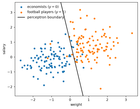
Fig. 94.1 Perceptron boundary separating the two groups#
Both boundaries point close to Fisher’s direction: the perceptron’s is about 11.5 degrees away and logistic regression’s about 4.
The closeness is no accident.
If the two classes are Gaussian with a common covariance matrix \(\Sigma\), then \(\Pr(y = 1 \mid x)\) is exactly a sigmoid in \(x\) whose slope is \(\Sigma^{-1}(\mu_1 - \mu_0)\), Fisher’s direction, so both recursions aim at it.
Here the two covariance matrices differ a little and the sample is finite, and the least squares criterion weights the observations differently from the likelihood, so the directions differ.
Minsky and Papert’s famous critique [Minsky and Papert, 1969] was precisely that a single perceptron can represent only a linear discriminant, and so cannot separate classes that a line cannot.
The revival of the field came with the recognition that layering perceptrons, feeding their outputs into further perceptrons, approximates any nonlinear discriminant, the subject of Introduction to Artificial Neural Networks.
For our purposes the perceptron is the entry in the catalogue closest to what the previous lectures already did: a parametric rule, trained by a stochastic-gradient recursion, that an econometrician would recognize on sight.
The Hopfield network is a bridge of another kind, and the last two brains are stranger still.
94.3. Associative memory: the Hopfield network#
The second device stores patterns and recalls them from corrupted fragments.
Represent a pattern as a vector of \(\pm 1\) of length \(N\).
We want to store \(p\) patterns \(\sigma^1, \ldots, \sigma^p\), the columns of an \(N \times p\) matrix \(\sigma\), so that each is a fixed point of a dynamical system, and so that feeding in a corrupted version converges quickly to the nearest stored pattern.
The Hopfield network [Hopfield, 1982] does this with the dynamics
and a weight matrix built from the patterns themselves.
When the patterns are orthogonal, Hebb’s rule \(w = \tfrac{1}{N}\sigma\sigma^\top\) suffices; for merely linearly independent (correlated) patterns one uses the projection rule \(w = \tfrac{1}{N}\sigma V^{-1}\sigma^\top\) with \(V = \tfrac{1}{N}\sigma^\top \sigma\).
Both make each stored pattern an exact fixed point.
The projection rule has a simple geometry: \(w = \sigma(\sigma^\top\sigma)^{-1}\sigma^\top\) is the orthogonal projection onto the span of the stored patterns.
So the energy \(E(s) = -\tfrac{1}{2}s^\top w s\) equals \(-\tfrac{1}{2}\lVert w s\rVert^2\), which is at least \(-\tfrac{1}{2}\lVert s\rVert^2 = -N/2\), with equality exactly when \(s\) lies in that span.
The stored patterns are therefore global minima of the energy.
We store five letters on a \(5\times5\) pixel grid, and because letters share many pixels, they are correlated, so the projection rule is the right one.
(The code stores the patterns as the rows of σ, the transpose of the matrix in the formulas.)
PATTERNS = {
    'A': ["01110", "10001", "11111", "10001", "10001"],
    'E': ["11111", "10000", "11110", "10000", "11111"],
    'I': ["11111", "00100", "00100", "00100", "11111"],
    'O': ["01110", "10001", "10001", "10001", "01110"],
    'T': ["11111", "00100", "00100", "00100", "00100"],
}

def to_vector(rows):
    return np.array([1 if c == '1' else -1 for r in rows for c in r])

letters = list(PATTERNS)
σ = np.array([to_vector(PATTERNS[c]) for c in letters])      # (p, N): one pattern per row

def projection_rule(patterns):
    "Weight matrix making each (correlated) pattern an exact fixed point."
    N = patterns.shape[1]
    Σ = patterns.T                                          # (N, p)
    V = Σ.T @ Σ / N
    return Σ @ np.linalg.inv(V) @ Σ.T / N

def energy(w, s):
    "Hopfield energy; stored patterns are global minima."
    return -0.5 * s @ w @ s

def recall(w, s0, max_iter=30):
    "Iterate sgn(w s) to a fixed point."
    s = s0.copy()
    for _ in range(max_iter):
        s_new = np.sign(w @ s)
        s_new[s_new == 0] = 1
        if np.array_equal(s_new, s):
            break
        s = s_new
    return s

w_hop = projection_rule(σ)
fixed = all(np.array_equal(np.sign(w_hop @ σ[i]), σ[i]) for i in range(len(letters)))
print(f"all stored letters are fixed points: {fixed}")
print(f"energy of each stored letter: {[round(energy(w_hop, σ[i]), 1) for i in range(len(letters))]}")
all stored letters are fixed points: True
energy of each stored letter: [np.float64(-12.5), np.float64(-12.5), np.float64(-12.5), np.float64(-12.5), np.float64(-12.5)]
Every stored letter sits at the same energy \(-N/2\) and is a fixed point.
Now corrupt a few pixels and let the network fall back to the nearest memory.
rng = np.random.default_rng(3)
show = ['E', 'O', 'T']

fig, axes = plt.subplots(len(show), 3, figsize=(6, 6))
for row, letter in enumerate(show):
    i = letters.index(letter)
    corrupt = σ[i].copy()
    corrupt[rng.choice(25, 4, replace=False)] *= -1             # flip 4 pixels
    recovered = recall(w_hop, corrupt)
    for col, (img, title) in enumerate([(σ[i], "stored"),
                                        (corrupt, "corrupted"),
                                        (recovered, "recovered")]):
        axes[row, col].imshow(img.reshape(5, 5), cmap='binary', vmin=-1, vmax=1)
        axes[row, col].set_xticks([])
        axes[row, col].set_yticks([])
        if row == 0:
            axes[row, col].set_title(title)
plt.tight_layout()
plt.show()
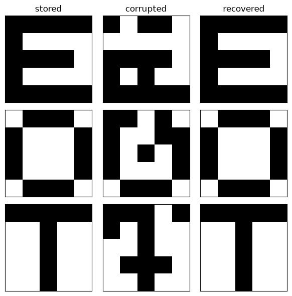
Fig. 94.2 Hopfield recall of letters from corrupted inputs#
The corrupted letters snap back to their originals.
How reliably depends on how much is corrupted and on how correlated the patterns are.
A corrupted letter can occasionally land in a different letter’s basin, or in a spurious mixture the designer never stored.
for n_flip in (3, 5, 7):
    correct = 0
    for i in range(len(letters)):
        for _ in range(40):
            corrupt = σ[i].copy()
            corrupt[rng.choice(25, n_flip, replace=False)] *= -1
            if np.array_equal(recall(w_hop, corrupt), σ[i]):
                correct += 1
    print(f"{n_flip} pixels flipped: recovered exactly {correct}/{len(letters)*40}")
3 pixels flipped: recovered exactly 179/200
5 pixels flipped: recovered exactly 138/200
7 pixels flipped: recovered exactly 77/200
Five patterns on 25 pixels is a heavy load (\(p/N = 0.2\)), and the letters overlap a lot: I and T differ in only 4 of the 25 pixels.
That is why even 3-pixel corruptions fail about one time in ten.
The book’s analysis of recall assumes many fewer patterns than pixels, \(p \ll N\).
The mechanism is worth naming because it recurs throughout this program.
Recall is descent on an energy function whose minima include the stored patterns.
Feeding in a corrupted pattern places the system on the energy surface near the right minimum, and the dynamics roll it down.
This is exactly the geometry behind simulated annealing, the method the book invokes for escaping unwanted local minima: add a controlled amount of random “shaking,” large at first and declining over time, so the system can hop out of shallow spurious basins before settling into a deep one.
Annealing and stochastic Newton methods modify Newton’s method to improve its global behavior without giving up its good local behavior.
The same principle, to experiment a lot early and less later, governs the classifier systems of Money as a Medium of Exchange among Artificially Intelligent Agents, whose genetic algorithm fires with a probability that declines like \(1/\sqrt{t}\), and the softmax auction of Exercise 94.3, whose “temperature” \(1/\beta\) plays the role of the shaking.
94.4. The genetic algorithm#
The third brain departs from Newton’s method more fundamentally: it does not descend a smooth surface at all.
Holland’s genetic algorithm [Goldberg, 1989, Holland, 1975] searches “rugged landscapes” that lack the smoothness Newton’s method needs, by evolving a population of candidate solutions encoded as binary strings.
The two approaches can be combined.
Ellen McGrattan applied genetic algorithms to estimate nonlinear rational expectations models: she first used a genetic algorithm to search for the vicinity of a maximum, then switched to a Newton method [Sargent, 1993].
The algorithm is handed two things: a nonnegative fitness function \(f\) to maximize, and an encoding that maps each binary string of length \(S\) to a candidate solution \(x\).
Given a population of \(N\) strings, one generation applies four operators:
Evaluation: compute each string’s fitness \(f(x_i)\).
Reproduction: copy strings into the next generation, string \(i\) with probability \(f(x_i)/\sum_j f(x_j)\), proportional to fitness (a “biased roulette wheel”).
Crossover: pair strings up and swap their tails at a random cut point, forming children that recombine their parents’ segments.
Mutation: flip each bit independently with a small probability \(p_m\).
The parameters of the algorithm are \(N\), \(S\) and \(p_m\).
Our code below uses a common variant of reproduction called windowing: it subtracts the generation’s lowest fitness before spinning the wheel.
When all fitnesses lie close together, as they will below, plain proportional selection barely discriminates among strings; windowing sharpens it, and gives the worst string essentially no chance to reproduce.
Reproduction concentrates the population on what already works; crossover and mutation inject new candidates.
Holland’s account of why crossover helps is in terms of schemata.
A schema \(H\) is a template in \(\{0, 1, *\}^S\), where \(*\) matches either bit: 1**0* is the set
of strings of length 5 with a 1 in the first position and a 0 in the fourth.
Its order \(o(H)\) is the number of fixed positions, and its defining length \(\delta(H)\) is the distance between the first and the last of them.
Holland’s schema theorem says that with fitness-proportional reproduction, single-point crossover applied to every pair, and mutation at rate \(p_m\), the expected number of strings in \(H\) satisfies
where \(f(H)\) is the average fitness of the strings in \(H\) and \(\bar f\) that of the whole population (with windowing, read \(f\) as the windowed fitness).
Short, low-order schemata with above-average fitness therefore tend to multiply.
The bound covers one generation only.
The “building-block hypothesis,” that the algorithm works by assembling short, fit schemata into better strings, is a heuristic rather than a theorem.
Whether it applies depends, in the book’s words, “precisely on how a given problem has been encoded”: on whether bits that work well together sit near one another.
The \(*\) of a schema reappears as the \(\#\) of a classifier’s condition below.
Crucially, the individual strings do not learn: each lives one generation and dies.
Only the society, the sequence of populations, learns.
(Arifovic’s election operator in Exchange Rate Indeterminacy, Learning, and Experiments softens this: a parent survives unless its child would have done better, so a good string can live for many generations.)
That is what makes the genetic algorithm awkward as a model of one brain, and a better fit as a model of a population or a market, a point that matters when we reach Money as a Medium of Exchange among Artificially Intelligent Agents.
94.4.1. Axelrod’s iterated prisoner’s dilemma#
Axelrod [1987] used the genetic algorithm to evolve strategies for the iterated prisoner’s dilemma, the game whose round-robin computer tournament, famously, was won by tit-for-tat.
He bred strategies against eight strategies representative of those submitted to his second tournament; we use a smaller panel.
Two players each choose to Cooperate or Defect; the payoffs reward defection against a cooperator but punish mutual defection.
# 1 = Cooperate, 0 = Defect;  T > R > P > S is the prisoner's dilemma ranking
T_pay, R_pay, P_pay, S_pay = 5, 3, 1, 0
PAYOFF = np.array([[P_pay, T_pay],       # row: my move (D, C); column: opponent's (D, C)
                   [S_pay, R_pay]])
Following Axelrod, a strategy is a 70-bit string: a strategy conditions on the outcomes of the last three rounds.
Each round is one of four outcomes (my move, opponent’s move), so three rounds give \(4^3 = 64\) possible histories, and 64 bits specify the action in each.
The remaining 6 bits encode a presumed pre-game history to get the first moves going.
Our play function plays a whole population of strings at once, one row per string.
POW = 2 ** np.arange(5, -1, -1)          # reads 6 history bits as an integer 0..63

def play(pop, opponent, n_rounds=150):
    "Play every 70-bit string in pop against opponent; return average payoffs."
    pop = np.atleast_2d(pop)
    N = len(pop)
    action = pop[:, :64]
    idx = pop[:, 64:] @ POW                       # the presumed pre-game history
    mine = np.zeros((N, n_rounds), int)
    theirs = np.zeros((N, n_rounds), int)
    my_total, opp_total = np.zeros(N), np.zeros(N)
    for t in range(n_rounds):
        a = action[np.arange(N), idx]             # my move from the lookup table
        b = opponent(mine[:, :t], theirs[:, :t], t)
        my_total += PAYOFF[a, b]
        opp_total += PAYOFF[b, a]
        mine[:, t], theirs[:, t] = a, b
        idx = 32 * a + 16 * b + (idx >> 2)        # newest round in, oldest round out
    return my_total / n_rounds, opp_total / n_rounds
The strategy is bred to do well against a fixed panel of opponents.
Each panel member is a function of the histories as that member sees them: its first argument is what its opponent has played and its second is what it has played itself.
The Random member flips a fair coin each round.
To make comparisons fair, each generation draws one sequence of coin flips, and every string in the population faces that same sequence.
This device, common random numbers, makes differences in fitness within a generation reflect differences in strategy rather than luck of the draw.
def all_cooperate(opp_moves, own_moves, t): return np.ones(len(opp_moves), int)
def all_defect(opp_moves, own_moves, t):    return np.zeros(len(opp_moves), int)

def tit_for_tat(opp_moves, own_moves, t):
    return opp_moves[:, -1] if t > 0 else np.ones(len(opp_moves), int)

def grudger(opp_moves, own_moves, t):
    return opp_moves.all(axis=1).astype(int)     # cooperate until the first defection

def random_opponent(flips):
    "An opponent who plays coin flips drawn in advance: row k of flips in game k."
    return lambda opp_moves, own_moves, t: flips[:, t]

PANEL = {'AllC': all_cooperate, 'AllD': all_defect,
         'TFT': tit_for_tat, 'Grudger': grudger}

def fitness(pop, flips):
    "Average payoff of each string against the panel, Random included."
    opponents = list(PANEL.values()) + [random_opponent(flips)]
    return np.mean([play(pop, opp)[0] for opp in opponents], axis=0)
Tit-for-tat copies what its opponent last did, and the grudger defects forever once its opponent has defected once.
Both are themselves 70-bit strings.
Tit-for-tat’s table copies the opponent’s most recent move.
The grudger’s table cooperates only after three rounds of mutual cooperation, which, starting from a cooperative pre-game history, is the same as never having seen a defection.
We use these two strings as benchmarks, and score any string by its payoff against each panel member, averaging over 400 fresh Random games (the same 400 for every string we compare).
TFT_GENE = np.r_[(np.arange(64) >> 4) & 1, np.ones(6, int)]
GRUDGER_GENE = np.r_[(np.arange(64) == 63).astype(int), np.ones(6, int)]

def panel_scores(gene, reps=400, seed=1):
    "Payoff against each panel member; Random is averaged over reps fresh games."
    flips = np.random.default_rng(seed).integers(0, 2, (reps, 150))
    scores = {name: play(gene, opp)[0][0] for name, opp in PANEL.items()}
    scores['Random'] = play(np.tile(gene, (reps, 1)), random_opponent(flips))[0].mean()
    return scores

def panel_fitness(gene):
    return np.mean(list(panel_scores(gene).values()))

def first_move(gene):
    return 'C' if gene[:64][gene[64:] @ POW] else 'D'
Now evolve.
We display one run, with seed 16, chosen because its champion’s fitness is close to the median of the twenty runs examined below.
def evolve(N=60, generations=80, p_mut=0.01, seed=0):
    rng = np.random.default_rng(seed)
    pop = rng.integers(0, 2, (N, 70))
    best_hist, mean_hist = [], []
    for _ in range(generations):
        flips = rng.integers(0, 2, (1, 150))           # one coin sequence for everyone
        fit = fitness(pop, flips)
        best_hist.append(fit.max())
        mean_hist.append(fit.mean())
        weight = fit - fit.min() + 1e-6                # windowing
        cum = np.cumsum(weight)
        parents = pop[np.searchsorted(cum, rng.random(N) * cum[-1])]
        mom, dad = parents[0::2], parents[1::2]
        left = np.arange(70) < rng.integers(1, 70, (N // 2, 1))   # single-point cuts
        pop = np.vstack([np.where(left, mom, dad), np.where(left, dad, mom)])
        pop[rng.random(pop.shape) < p_mut] ^= 1        # mutation
    fit = fitness(pop, rng.integers(0, 2, (1, 150)))
    return pop[fit.argmax()], np.array(best_hist), np.array(mean_hist)


champion, best_hist, mean_hist = evolve(seed=16)
print(f"generation 0:  best {best_hist[0]:.3f}, mean {mean_hist[0]:.3f}")
print(f"generation {len(best_hist)-1}: best {best_hist[-1]:.3f}, mean {mean_hist[-1]:.3f}")
generation 0:  best 2.429, mean 1.941
generation 79: best 2.608, mean 2.397
The figure tracks the best and the mean fitness within each generation.
fig, ax = plt.subplots(figsize=(7.5, 4))
ax.plot(best_hist, label="best in population", lw=2)
ax.plot(mean_hist, label="population mean", lw=2)
ax.set_xlabel("generation")
ax.set_ylabel("panel fitness")
ax.legend(frameon=False)
plt.show()
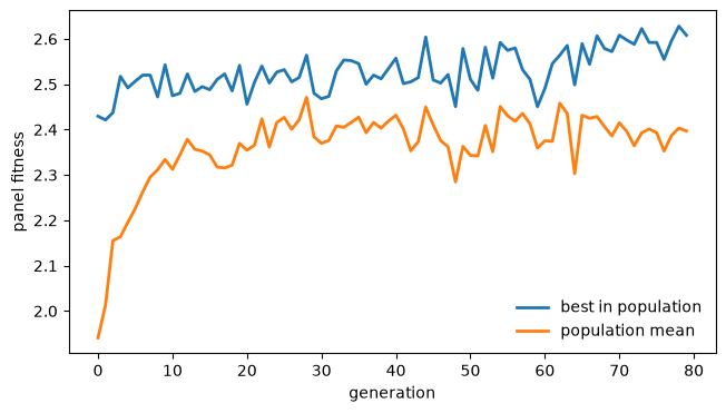
Fig. 94.3 Population fitness across generations#
The population mean climbs quickly for about a dozen generations and then fluctuates around 2.4, held down by the crossover and mutation that keep creating weaker strings.
The best string’s fitness jumps around and drifts up slowly, to about 2.6 by the end.
It jumps around because each generation faces a new sequence of coin flips from Random, and because nothing guarantees that the best string survives reproduction, crossover, and mutation.
What kind of strategy did evolution find?
strategies = {'champion': champion, 'TFT': TFT_GENE, 'Grudger': GRUDGER_GENE}
table = {name: panel_scores(gene) for name, gene in strategies.items()}

print(f"{'payoff vs':>10}" + "".join(f"{name:>10}" for name in strategies))
for opp in table['champion']:
    print(f"{opp:>10}" + "".join(f"{table[name][opp]:>10.3f}" for name in strategies))
print(f"{'panel avg':>10}" + "".join(f"{np.mean(list(table[name].values())):>10.3f}"
                                     for name in strategies))
print(f"champion's first move: {first_move(champion)}")
 payoff vs  champion       TFT   Grudger
      AllC     3.000     3.000     3.000
      AllD     0.987     0.993     0.993
       TFT     3.000     3.000     3.000
   Grudger     3.000     3.000     3.000
    Random     2.881     2.239     2.971
 panel avg     2.573     2.446     2.593
champion's first move: C
The evolved strategy is nice, in Axelrod’s language: it is never the first to defect against AllC, TFT, or the grudger, and so earns the mutual-cooperation payoff of 3 against all three.
It refuses to be suckered by AllD after its first two rounds, and it defects against Random often enough to earn much more than tit-for-tat does.
Against this panel it beats tit-for-tat, and the margin comes almost entirely from Random.
It does not beat the grudger, a member of the panel, which does slightly better still.
Is this run typical?
The next cell repeats the experiment with twenty seeds.
results = []
for seed in range(20):
    sc = panel_scores(evolve(seed=seed)[0])
    nice = all(sc[k] == 3.0 for k in ('AllC', 'TFT', 'Grudger'))
    results.append((np.mean(list(sc.values())), nice))
fits = np.array([r[0] for r in results])
nice = np.array([r[1] for r in results])
tft_fit, grudger_fit = panel_fitness(TFT_GENE), panel_fitness(GRUDGER_GENE)

print(f"nice champions: {nice.sum()} of 20")
print(f"champion fitness: median {np.median(fits):.3f}, "
      f"range [{fits.min():.3f}, {fits.max():.3f}]")
print(f"  nice ones: mean {fits[nice].mean():.3f};  others: mean {fits[~nice].mean():.3f}")
print(f"beat TFT ({tft_fit:.3f}): {np.sum(fits > tft_fit)} of 20")
print(f"within 0.01 of Grudger ({grudger_fit:.3f}): {np.sum(fits > grudger_fit - 0.01)} of 20;"
      f"  above it: {np.sum(fits > grudger_fit)}")
nice champions: 15 of 20
champion fitness: median 2.576, range [2.481, 2.594]
  nice ones: mean 2.550;  others: mean 2.556
beat TFT (2.446): 20 of 20
within 0.01 of Grudger (2.593): 7 of 20;  above it: 1
Most champions are nice, but not all.
The rest are probe-and-exploit strategies: at some point they defect unprovoked, which wins 5 a round forever against AllC and plunges them into mutual defection with the grudger.
The panel makes the two families almost exactly equal.
AllC and the grudger behave identically until someone defects, so a strategy cannot tell them apart without probing.
A probe gains 2 a round against AllC and loses 2 a round against the grudger, so the two families tie on that pair of opponents.
Which family the algorithm lands on is a matter of the seed: a small instance of a rugged landscape with two peaks of almost equal height.
The panel also has a ceiling.
No strategy can average more than 1 against AllD, more than 3 against Random (against a coin, defection is better whatever the coin shows), more than about 3 against tit-for-tat, or more than about 6 against AllC and the grudger together.
So panel fitness cannot exceed about \(13/5 = 2.6\), and the grudger is already within 0.01 of that ceiling.
Every champion beats tit-for-tat, but none beats the grudger by more than a rounding error.
Axelrod’s own genetic algorithm, as Sargent [1993] summarizes it, “produced a strategy that would have won the tournament, and in particular would have outplayed the ‘tit-for-tat’ strategy that won the tournament.”
Our toy version reproduces the second half of that sentence, and shows where the edge comes from.
It is not extra memory: the grudger needs only one bit of memory, and does as well as any champion.
It is refusing to forgive: against Random, tit-for-tat keeps returning to cooperation and gets suckered, while the grudger and the best champions settle into defection.
And, as Sargent notes, such comparisons flatter the genetic algorithm, because it “got to practice against” its opponents, while the strategies submitted to a tournament could only guess what they would face.
94.5. Classifier systems#
The genetic algorithm evolves a population in which no individual learns.
Holland’s classifier system puts the same evolutionary machinery inside a single agent, as a model of one brain [Holland et al., 1986].
Sargent describes it as Holland’s vision of the mind as a competitive economy:
The statements compete with one another for the opportunity to decide. The classifier system incorporates elements of the genetic algorithm with other aspects in a way that represents a brain in terms that Holland describes as a competitive economy.
A classifier system has five parts:
Classifiers, if-then rules encoded as strings over the trinary alphabet \(\{0, 1, \#\}\), with a condition part that is matched against the state and an action part that prescribes a move.
A decoder that, given the current state, finds which classifiers’ conditions match.
An auction that selects one matching classifier to act.
An accounting system that updates each classifier’s strength from the payoffs that follow its decisions and, in sequential problems, passes payoffs backward along the chain of rules that produced them.
A device for creating new classifiers, so that the system’s very vocabulary evolves:
when no classifier matches the state, one is created whose condition matches it and whose action is random;
now and then new rules replace weak ones, so that untried actions get tried;
rules are generalized (0’s and 1’s replaced by \(\#\)’s) or specialized (\(\#\)’s replaced by 0’s and 1’s), often by genetic operators.
We take the decoder and the auction first, then the accounting system, through two examples: the bandit and the bucket brigade.
94.5.1. Matching, specificity, and bids#
A state matches a condition if they agree in every position where the condition does not have a \(\#\), the “I don’t care” symbol.
The condition 1#0 matches the states 100 and 110 and nothing else.
A rule with many \(\#\)’s is general: its condition is met often.
A rule with few is specific.
Marimon et al. [1990] measure the specificity of a classifier \(e\) by \(\sigma_e = 1/(1 + \text{number of } \#\text{'s in } e)\).
def matches(condition, state):
    "A state matches if it agrees with every position that is not '#'."
    return all(c in ('#', s) for c, s in zip(condition, state))

def specificity(condition):
    return 1 / (1 + condition.count('#'))

state = '110'
for condition in ('110', '1#0', '##0', '###', '0##'):
    print(f"condition {condition}: matches {state}? {str(matches(condition, state)):5}  "
          f"specificity {specificity(condition):.2f}")
condition 110: matches 110? True   specificity 1.00
condition 1#0: matches 110? True   specificity 0.50
condition ##0: matches 110? True   specificity 0.33
condition ###: matches 110? True   specificity 0.25
condition 0##: matches 110? False  specificity 0.33
Several rules usually match at once, and they may disagree about what to do.
Each matched rule \(e\) bids a fraction \(b(e)\) of its strength \(S_e\), a fraction that rises with its specificity:
where, in the notation of Marimon et al. [1990], \(b_{11}\) and \(b_{12}\) are positive constants that sum to less than one.
When a general rule and a specific one are equally strong, the specific one outbids it, so an auction on bids favors it.
This is how a classifier system handles the trade-off that the book calls generality versus discrimination.
General rules are tested often, because their conditions are often met, but they prescribe the same action across many states.
Specific rules can fit the action to the state, but they need long histories before their strengths mean much.
The trade-off resembles the one between parametric and non-parametric estimation (Learning without a functional form).
With a specificity premium, a specific rule can carve out an exception to a general one, and the balance between generality and specificity can itself evolve as rules are generalized and specialized.
94.5.2. The auction#
The auction turns bids into a decision.
The book lists two principles: the highest bidder wins, or each matched rule wins with probability equal to its relative strength.
Both belong to one family, the softmax:
where \(M\) is the set of matched rules.
As \(\beta \to \infty\) the softmax puts all its weight on the highest bid, so the argmax auction is its limit.
Applied to the logarithms of strengths with \(\beta = 1\), it gives the relative-strength rule, since \(\exp(\ln S_e) / \sum_{e'} \exp(\ln S_{e'}) = S_e / \sum_{e'} S_{e'}\).
The parameter \(\beta\) sets how much the system experiments.
The argmax auction never lets a rule that looks worse act, so it can never discover that the rule is in fact better; with a finite \(\beta\), the system always might.
Money as a Medium of Exchange among Artificially Intelligent Agents uses an argmax auction applied to strengths rather than bids: there the strongest matched rule acts, bids only set the payments of the bucket brigade, and all experimentation is left to the operators for creating rules.
94.5.3. A two-armed bandit#
The simplest classifier system is an example of Brian Arthur and Carl Simon, who presented it independently at the Santa Fe Institute in 1989 (see also Arthur [1991]).
Arm \(i\) pays a random reward with mean \(\mu_i > 0\), with \(\mu_1 > \mu_2\), and the player knows neither distribution.
The classifier system holds two rules, #1 (“whatever the history, pull arm 1”) and #0
(“pull arm 2”), whose conditions are always met.
Arthur’s accounting sets the strength of rule \(i\) to the average payoff its arm has delivered,
where \(\tau_i\) counts the times arm \(i\) has been pulled, and the auction picks rule \(i\) with probability \(S_i / (S_1 + S_2)\).
The two rules start with equal strengths: the system is told nothing about either arm and must build its estimates out of the rewards it experiences.
def two_armed_bandit(μ, noise_sd=0.5, T=20_000, seed=0):
    "Strength = running average of an arm's payoff; pull ∝ strength."
    rng = np.random.default_rng(seed)
    S = np.ones(2)                             # equal strengths: no prior knowledge
    τ = np.array([1, 1])                       # pull counters
    pulls = np.empty(T, int)
    for t in range(T):
        w = np.maximum(S, 1e-9)                # guard against a dip below zero
        i = 0 if rng.random() < w[0] / w.sum() else 1
        reward = μ[i] + noise_sd * rng.standard_normal()
        τ[i] += 1
        S[i] += (reward - S[i]) / τ[i]         # running average
        pulls[t] = i
    return pulls

pulls = two_armed_bandit([3.0, 1.0])
frac_best = np.cumsum(pulls == 0) / np.arange(1, len(pulls) + 1)

fig, ax = plt.subplots(figsize=(7.5, 4))
ax.plot(frac_best, lw=1)
ax.axhline(0.75, color='k', ls='--', label="probability match  $\\mu_1/(\\mu_1+\\mu_2)$")
ax.axhline(1.0, color='C3', ls=':', label="optimal (always best arm)")
ax.set_xlabel("$t$")
ax.set_ylabel("fraction of pulls on the best arm")
ax.set_ylim(0.5, 1.05)
ax.legend(frameon=False)
plt.show()
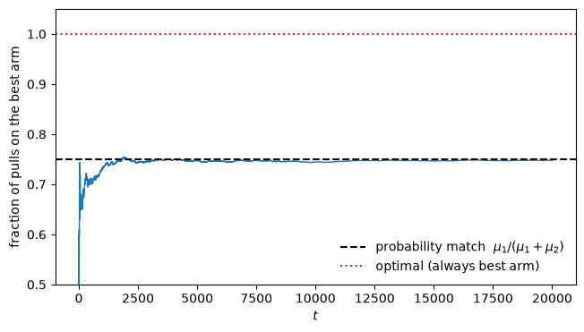
Fig. 94.4 The classifier bandit converges to probability matching#
The fraction of pulls on the better arm converges, but not to one.
It converges to \(\mu_1/(\mu_1 + \mu_2)\), the arm’s share of total expected reward.
for μ in ([1.0, 0.5], [2.0, 1.0], [3.0, 1.0]):
    frac = np.mean(two_armed_bandit(μ)[-5000:] == 0)
    print(f"μ = {μ}: fraction on best arm = {frac:.3f}, "
          f"probability match = {μ[0]/(μ[0]+μ[1]):.3f}  (optimal = 1.0)")
μ = [1.0, 0.5]: fraction on best arm = 0.655, probability match = 0.667  (optimal = 1.0)
μ = [2.0, 1.0]: fraction on best arm = 0.659, probability match = 0.667  (optimal = 1.0)
μ = [3.0, 1.0]: fraction on best arm = 0.750, probability match = 0.750  (optimal = 1.0)
Arthur showed, by the methods of stochastic approximation, that the strength-proportional classifier probability-matches.
The argument is short.
As long as the strengths stay positive, which needs \(\mu_i > 0\), each arm keeps a positive probability of being pulled, and so is pulled infinitely often.
Each strength is the sample mean of its arm’s payoffs, so it converges to \(\mu_i\) by the strong law of large numbers.
The auction’s probabilities therefore converge to \(\mu_1/(\mu_1 + \mu_2)\), and so does the fraction of pulls on arm 1.
The classifier plays the arms in proportion to their expected rewards rather than concentrating on the best one, so it leaves reward on the table forever.
With \(\mu = (3, 1)\) it earns \(0.75 \times 3 + 0.25 \times 1 = 2.5\) a pull, against 3 for always pulling arm 1.
The proportional rule also cares only about the ratio \(\mu_1/\mu_2\): \(\mu = (1, 0.5)\) and \(\mu = (2, 1)\) produce the same shares.
Notice where the trouble lies.
The accounting is fine: each strength converges to the right number, its arm’s mean payoff.
The trouble is the auction, which turns correct strengths into choice probabilities proportional to them.
Exercise 94.3 cures probability matching by changing the auction alone.
That separates two jobs.
The auction governs the balance between exploring and exploiting.
The accounting governs credit assignment, which is trivial in the bandit, where each payoff belongs to the arm that produced it, but hard in sequential problems.
94.5.4. The bucket brigade#
In a sequential problem, a rule’s decision may pay off only later, through a chain of further decisions.
The accounting must then reward a rule for merely setting up a profitable future decision.
Holland’s device for this is the bucket brigade: each rule that wins an auction pays its bid to the rule that acted just before it, the one that moved the system into the state where the current rule could act.
A rule’s receipts are the payoff it collects from the environment plus the bid paid to it by its successor.
Take the shortest chain.
A setup rule \(s\) acts first and moves the system into a state where a payoff rule \(p\) acts and collects \(R\).
Rule \(p\) pays its bid \(b S_p\) back to \(s\); to keep things simple, every rule bids the same fraction \(b\) of its strength.
Holland kept strengths as cumulative balances: a rule that acts pays out its bid and takes in its receipts, like a bank account, so that \(S \leftarrow S - bS + \text{receipts}\).
Arthur, in the bandit, and Marimon et al. [1990], in the economy of the next lecture, average instead:
where \(\tau\) counts the times the rule has acted, so that strength is a running average of receipts net of the bid.
With \(b = 0\) this is the bandit’s running average.
The code runs both accountings on the chain, starting from zero strengths, with \(R = 1\) and \(b = 0.1\).
def bucket_brigade(R=1.0, b=0.1, passes=10_000, accounting='average'):
    "Two-link chain: the setup rule acts, then the payoff rule acts and earns R."
    S = np.zeros(2)                                # strengths of [setup, payoff]
    path = []
    for τ in range(1, passes + 1):
        receipts = np.array([b * S[1], R])         # the payoff rule pays its bid back
        if accounting == 'average':                # Arthur; Marimon-McGrattan-Sargent
            S = S + (receipts - (1 + b) * S) / τ
        else:                                      # Holland's cumulative balance
            S = S - b * S + receipts
        path.append(S.copy())
    return np.array(path)

for accounting in ('balance', 'average'):
    path = bucket_brigade(accounting=accounting)
    print(f"{accounting}: [setup, payoff] after passes 1, 2, 3: "
          f"{path[0].round(3)}, {path[1].round(3)}, {path[2].round(3)};  "
          f"limit {path[-1].round(3)}")
balance: [setup, payoff] after passes 1, 2, 3: [0. 1.], [0.1 1.9], [0.28 2.71];  limit [10. 10.]
average: [setup, payoff] after passes 1, 2, 3: [0. 1.], [0.05 0.95], [0.063 0.935];  limit [0.083 0.909]
Two things stand out.
First, credit moves back one link per pass.
In the first pass the payoff rule collects \(R\) but the setup rule receives nothing, because the payoff rule’s strength, and hence its bid, was still zero when it paid.
In a chain of \(k\) links, the payoff takes \(k - 1\) passes to reach the first rule.
Second, the two accountings disagree about what the setup rule is worth.
Cumulative balances come to rest where receipts equal the bid, \(b S_p = R\) and \(b S_s = b S_p\), so \(S_s = S_p = R/b\): the setup rule ends up exactly as strong as the payoff rule.
Averages come to rest where \((1 + b)S_p = R\) and \((1 + b)S_s = b S_p\), so
Each link back along the chain scales strength by \(b/(1+b)\), about 0.09 when \(b = 0.1\).
The averaging accounting values a setup rule as if it discounted the future very heavily, a fact with large consequences in Money as a Medium of Exchange among Artificially Intelligent Agents (The bucket brigade’s discount factor).
Exercise 94.5 asks when a setup rule can beat a rule that pays off at once.
Why average, then?
Holland’s balance with bids proportional to strength can be written \(S \leftarrow S + b\,(\text{receipts}/b - S)\), a constant-gain average of receipts\(/b\), which keeps fluctuating as long as the receipts are random.
The \(1/\tau\) gain turns it into a decreasing-gain stochastic approximation of the kind studied in One recursion, many learners.
Its limit is a rest point of the mean dynamics \(dS/d\tau = \mathbb{E}[\text{receipts}] - (1 + b) S\), which is what makes strengths converge and lets the next lecture characterize their limits.
The bucket brigade is also an ancestor of temporal-difference learning [Sutton and Barto, 2018].
A rule’s strength is moved toward what it earns now plus a fraction of the strength of the rule it hands the system to.
The Q-learning of Job Search X: Search with Q-Learning and Inventory Management via Q-Learning moves the value of a state-action pair toward the current reward plus the discounted value of the next state in the same way, with the successor’s bid playing the role of that discounted value.
Designing that backward flow is the central craft of building a classifier system, and it is exactly what Money as a Medium of Exchange among Artificially Intelligent Agents must get right to make agents learn to accept money today for the sake of a trade tomorrow.
94.6. Evolutionary programming#
We have surveyed four brains.
The last idea is about what to do with them.
Many of the systems of adaptive agents in this series, however plodding, find their way to an equilibrium.
The least squares learners of Adaptive Agents in an Overlapping Generations Monetary Economy converge to a stationary equilibrium, and the learners of Learning, Approximation, and Equilibrium Computation to the best approximate equilibrium their functional form allows.
At Sargent’s calibration, the Newton learners of Exchange Rate Indeterminacy, Learning, and Experiments converge to one of a continuum of equilibria, picked out by history.
Not all of them do.
The same Newton learners fail to converge at Arifovic’s calibration.
And the genetic-algorithm economy of Exchange Rate Indeterminacy, Learning, and Experiments never settles down (A genetic algorithm economy): its saving rate settles near the equilibrium value, but mutation keeps injecting new strings, and its exchange rate keeps fluctuating with a volatility that does not die out.
Evolutionary programming turns the tendency to converge into a tool.
If a population of adaptive agents reliably converges to an equilibrium, we can run the population as a method for computing the equilibrium, especially in models too complicated to solve by hand.
The genetic-algorithm economy is a reminder that the reliability has to be designed in: the experimentation must die away, as annealing’s shaking does, if the population is to come to rest.
Sargent is careful about what is and isn’t going on:
The adaptive agents are ‘teaching’ the economist in the same sense that any numerical algorithm for solving nonlinear equations ‘teaches’ a mathematician. When these agents can ‘teach’ us something, it is because we designed them to do so.
This is the same duality that ran through Learning, Approximation, and Equilibrium Computation: a learning economy is a decentralized equilibrium computation, and an equilibrium computation is a centralized learning algorithm.
The genetic algorithm and the classifier system are simply richer computational engines than recursive least squares, able to search rugged landscapes and to discover the structure of a good rule, not just tune the coefficients of a fixed one.
The showcase is Kiyotaki and Wright [1989]’s search-theoretic model of money, in which the medium of exchange is not assumed but must emerge from how agents choose to trade.
The equilibrium is a set of trading strategies and matching probabilities, and for enriched versions of the model it is hard to characterize analytically.
Marimon et al. [1990] put populations of Holland classifier systems into that environment and watched them converge to an equilibrium, then built a five-good version, with no known analytical solution, and let the classifier systems suggest what the equilibrium looked like.
94.7. Concluding remarks#
The four brains in this catalogue differ in what they take as given.
The perceptron is handed a functional form and asked only for its coefficients, which is why an econometrician recognizes it immediately.
The Hopfield network is handed the patterns themselves and asked only to recall them.
The genetic algorithm is handed an encoding and a fitness function and must search a space in which it cannot compute a gradient.
The classifier system is handed a vocabulary in which rules can be written and must discover which rules are worth holding.
Moving down that list, we hand the agent less and ask it to find more, which is precisely the direction the bounded-rationality program pushes us.
Three cautions emerged along the way, and all three return in the next lecture.
The genetic algorithm’s individuals do not learn: only the population does, which makes it a model of a society rather than of a mind, and a population that never stops experimenting, as in Exchange Rate Indeterminacy, Learning, and Experiments, need not settle down.
The bandit showed that a classifier system’s behavior is decided by its auction and its accounting rather than by the fact of having classifiers at all: the auction decides how much it experiments, and the accounting how it assigns credit.
And the bucket brigade showed that the accounting builds in a valuation of the future: with averaged strengths, a rule that sets up a payoff one link away is worth only a fraction \(b/(1+b)\) of the rule that collects it.
Money as a Medium of Exchange among Artificially Intelligent Agents assembles this machinery into agents who must learn, from scratch, which good to use as money.
Their rules have conditions over \(\{0, 1, \#\}\) and bid in proportion to strength with a specificity premium; an argmax auction on strength picks among them; a bucket brigade links each trade to the consumption it makes possible; and a genetic algorithm whose activity dies away over time refreshes them.
All three cautions bear directly on what those agents turn out to be able to learn.
94.8. Exercises#
Exercise 94.1
The Hopfield network’s recall is descent on the energy \(E(s) = -\tfrac{1}{2}s^\top ws\).
Verify the descent directly.
Take a stored letter, corrupt several pixels, and record the energy at each step of the recall dynamics.
Confirm that energy never increases, and that a recall that ends at a stored letter ends at energy \(-N/2\), the lowest energy any state can have.
Then prove that energy cannot increase under the synchronous update \(s' = \operatorname{sgn}(ws)\) when \(w\) is the projection-rule matrix.
Finally, corrupt patterns more heavily and classify the failures: does recall land on a different stored letter, or on a spurious state that was never stored?
Compare the energies in each case, and use them to explain why the error happens.
Solution
Here is a version of recall that records the energy at every step.
def recall_with_energy(w, s0, max_iter=30):
    s = s0.copy()
    trace = [energy(w, s)]
    for _ in range(max_iter):
        s_new = np.sign(w @ s)
        s_new[s_new == 0] = 1
        trace.append(energy(w, s_new))
        if np.array_equal(s_new, s):
            break
        s = s_new
    return s, trace

rng = np.random.default_rng(1)
i = letters.index('E')
corrupt = σ[i].copy()
corrupt[rng.choice(25, 5, replace=False)] *= -1
final, trace = recall_with_energy(w_hop, corrupt)

print(f"energy along the recall path: {[round(e, 2) for e in trace]}")
print(f"monotonically non-increasing: {all(np.diff(trace) <= 1e-9)}")
print(f"recovered the intended letter 'E': {np.array_equal(final, σ[i])}")
energy along the recall path: [np.float64(-6.38), np.float64(-12.5), np.float64(-12.5)]
monotonically non-increasing: True
recovered the intended letter 'E': True
The energy falls from its corrupted value to \(-N/2 = -12.5\) and stays there.
Here is why it cannot rise.
Let \(s' = \operatorname{sgn}(ws)\) and \(d = s' - s\).
Expanding the quadratic form, and using the symmetry of \(w\),
Each nonzero entry of \(d\) is \(d_i = 2 s'_i = 2\operatorname{sgn}((ws)_i)\), so the first term is \(-2\sum_i |(ws)_i|\), summed over the flipped pixels, and is never positive.
The second term is never positive either, because the projection matrix \(w\) is positive semidefinite.
So the energy never rises, and it falls strictly whenever a pixel flips against a nonzero field.
Since there are finitely many states, recall cannot cycle and must halt at a fixed point.
(Ties are broken toward \(+1\), as in the code, so a pixel can only flip from \(+1\) to \(-1\) against a strictly negative field, and that strict fall rules out cycles.)
The argument uses positive semidefiniteness, which the projection rule has.
The usual Hebb rule with its diagonal set to zero does not have it, and with such weights, updating all pixels at once can cycle between two states.
Hopfield’s own energy argument [Hopfield, 1982] is for updating one pixel at a time.
Now corrupt more heavily and sort the outcomes into three kinds: the intended letter, a different stored letter, and a spurious state that is a fixed point but was never taught.
The code also checks monotonicity on every one of the 1000 recall paths, and looks at the spurious states that sit at the lowest possible energy.
def classify_outcome(final, i):
    if np.array_equal(final, σ[i]):
        return "intended"
    if any(np.array_equal(final, σ[k]) for k in range(len(letters))):
        return "wrong letter"
    return "spurious"

counts = {"intended": 0, "wrong letter": 0, "spurious": 0}
wrong_energy, spurious_energy, deepest = [], [], []
always_downhill = True
for i in range(len(letters)):
    for seed in range(200):
        r = np.random.default_rng(1000*i + seed)
        corrupt = σ[i].copy()
        corrupt[r.choice(25, 7, replace=False)] *= -1
        final, trace = recall_with_energy(w_hop, corrupt)
        always_downhill &= all(np.diff(trace) <= 1e-9)
        kind = classify_outcome(final, i)
        counts[kind] += 1
        if kind == "wrong letter":
            wrong_energy.append(energy(w_hop, final))
        elif kind == "spurious":
            spurious_energy.append(energy(w_hop, final))
            if np.isclose(energy(w_hop, final), -12.5):
                deepest.append(final)

negatives = sum(any(np.array_equal(s, -σ[k]) for k in range(len(letters))) for s in deepest)
print(f"7-pixel corruptions ({sum(counts.values())} trials): {counts}")
print(f"energy non-increasing on every path: {always_downhill}")
print(f"stored patterns all have energy {energy(w_hop, σ[0]):.1f}")
print(f"wrong-letter results: energy in [{min(wrong_energy):.1f}, {max(wrong_energy):.1f}]")
print(f"spurious results:     energy in [{min(spurious_energy):.1f}, {max(spurious_energy):.1f}]")
print(f"spurious results at energy -N/2: {len(deepest)}, "
      f"of which sign-reversed letters: {negatives}")
7-pixel corruptions (1000 trials): {'intended': 404, 'wrong letter': 62, 'spurious': 534}
energy non-increasing on every path: True
stored patterns all have energy -12.5
wrong-letter results: energy in [-12.5, -12.5]
spurious results:     energy in [-12.5, -10.4]
spurious results at energy -N/2: 41, of which sign-reversed letters: 3
Both failure modes occur, and at this level of corruption spurious states outnumber wrong letters by almost nine to one.
A wrong-letter result sits at exactly the stored energy \(-N/2\): the corruption pushed the starting point clear across a basin boundary, into the domain of attraction of a different stored memory that is just as deep.
Energy descent converges to a minimum but cannot guarantee the nearest one when correlated patterns have interlocking basins.
A spurious result is a fixed point the designer never intended, created as an artifact of the storage rule.
Most spurious results are shallower than the stored patterns: they are fixed points outside the span of the letters, most of them local minima.
A minority sit at exactly \(-N/2\), which requires them to lie in that span.
Some of those are photographic negatives of letters: because \(\operatorname{sgn}(w(-s)) = -\operatorname{sgn}(ws)\), the vector \(-\sigma\) is a fixed point whenever \(\sigma\) is.
Most are signed mixtures of letters that happen to be \(\pm 1\) vectors, such as \(E - I + T\) and \(A - E + I\).
Depth alone therefore does not identify a memory as one we asked for.
Because all of these are fixed points of the update, the dynamics cannot escape any of them.
That is why simulated annealing matters: adding declining random shaking lets the system hop out of a shallow spurious basin, or across a basin boundary, before settling, something pure energy descent can never do.
Exercise 94.2
The genetic algorithm’s exploration comes from two operators, crossover and mutation.
The book argues that crossover “lies at the heart of the algorithm,” while mutation alone “is a poor mechanism for injecting diversity.”
Test the claim on Axelrod’s game.
Write a mutation-only variant (each child is a mutated copy of one selected parent, with no crossover) and compare the fitness it reaches against the full algorithm.
Score each run by its champion’s panel_fitness, so that every strategy faces the same Random
games, and use several seeds.
The book is careful to say when mutation alone is weak: “when the mutation rate is set to a very low value, mutation alone is a poor mechanism for injecting diversity.”
So run the comparison at a low mutation rate, \(p_m = 0.002\), where crossover has to carry the exploration, and then at a higher one, \(p_m = 0.02\).
Solution
The mutation-only variant keeps the windowed roulette wheel and drops crossover.
def evolve_mutation_only(N=60, generations=60, p_mut=0.002, seed=0):
    "Each child is a mutated copy of one roulette-selected parent."
    rng = np.random.default_rng(seed)
    pop = rng.integers(0, 2, (N, 70))
    for _ in range(generations):
        fit = fitness(pop, rng.integers(0, 2, (1, 150)))
        weight = fit - fit.min() + 1e-6
        cum = np.cumsum(weight)
        pop = pop[np.searchsorted(cum, rng.random(N) * cum[-1])]
        pop[rng.random(pop.shape) < p_mut] ^= 1
    fit = fitness(pop, rng.integers(0, 2, (1, 150)))
    return pop[fit.argmax()]

n_seeds = 12
for p_mut in (0.002, 0.02):
    gaps = []
    for seed in range(n_seeds):
        with_x = panel_fitness(evolve(generations=60, p_mut=p_mut, seed=seed)[0])
        without_x = panel_fitness(evolve_mutation_only(p_mut=p_mut, seed=seed))
        gaps.append(with_x - without_x)
    gaps = np.array(gaps)
    print(f"p_mut = {p_mut}: crossover minus mutation-only = {gaps.mean():.3f} "
          f"(standard error {gaps.std(ddof=1) / np.sqrt(n_seeds):.3f}); "
          f"crossover ahead in {np.sum(gaps > 0)} of {n_seeds} seeds")
p_mut = 0.002: crossover minus mutation-only = 0.070 (standard error 0.017); crossover ahead in 11 of 12 seeds
p_mut = 0.02: crossover minus mutation-only = -0.010 (standard error 0.020); crossover ahead in 6 of 12 seeds
At the low mutation rate crossover clearly wins: its champion is fitter in almost every seed.
At the higher rate the advantage shrinks to near zero: in these seeds the average gap is within one standard error of zero, and crossover is ahead in only about half of them.
The reason is the one the book gives.
With little mutation, a mutation-only population can only inch forward one rare bit-flip at a time, and it quickly loses diversity as selection copies its few best strings.
Crossover instead recombines segments of strings that have already proved useful.
In this encoding a block of 16 consecutive table entries is a set of histories that share the most recent round’s outcome, so crossover splices one string’s responses to some recent outcomes onto another string’s responses to others.
That is the schema story, though the schema theorem guarantees only that short, fit blocks tend to survive, not that splicing them improves the string.
When mutation generates plenty of diversity on its own, crossover’s contribution is no longer pivotal, which is the book’s qualification: it is at a very low mutation rate that mutation alone is weak.
Exercise 94.3
The two-armed bandit classifier probability-matches, which is suboptimal: it keeps pulling the worse arm a fixed fraction of the time forever.
A natural fix is to make the auction greedier.
Replace the strength-proportional choice rule with a softmax,
where \(\beta\) controls greediness (\(\beta \to \infty\) always picks the stronger arm).
Implement it and show how the long-run fraction on the best arm depends on \(\beta\), for \(\mu = (3, 1)\).
How large must \(\beta\) be for the softmax to beat probability matching?
Now make the arms hard to tell apart: \(\mu = (1.2, 1.0)\) with reward noise of standard deviation 2. Compare \(\beta = 2\) with a very greedy \(\beta = 32\) across 40 seeds. What does greed cost?
Solution
The softmax bandit changes only the line that chooses the arm.
def bandit_softmax(μ, β, noise_sd=0.5, T=20_000, seed=0):
    "Share of the last 5000 pulls on arm 1 under a softmax auction."
    rng = np.random.default_rng(seed)
    S = np.ones(2)                             # equal strengths, as before
    τ = np.array([1, 1])
    pulls = np.empty(T, int)
    for t in range(T):
        p1 = 1 / (1 + np.exp(-β * (S[0] - S[1])))
        i = 0 if rng.random() < p1 else 1
        reward = μ[i] + noise_sd * rng.standard_normal()
        τ[i] += 1
        S[i] += (reward - S[i]) / τ[i]
        pulls[t] = i
    return np.mean(pulls[-5000:] == 0)

μ = [3.0, 1.0]
β_star = np.log(μ[0] / μ[1]) / (μ[0] - μ[1])
print(f"probability match target = {μ[0]/(μ[0]+μ[1]):.3f},  optimal = 1.000,  "
      f"break-even β = {β_star:.3f}\n")
for β in (0.5, 1.0, 2.0, 4.0, 8.0):
    theory = 1 / (1 + np.exp(-β * (μ[0] - μ[1])))
    print(f"β = {β:>4}: fraction on best arm = {bandit_softmax(μ, β):.3f}  "
          f"(limit {theory:.3f})")
probability match target = 0.750,  optimal = 1.000,  break-even β = 0.549

β =  0.5: fraction on best arm = 0.732  (limit 0.731)
β =  1.0: fraction on best arm = 0.888  (limit 0.881)
β =  2.0: fraction on best arm = 0.980  (limit 0.982)
β =  4.0: fraction on best arm = 1.000  (limit 1.000)
β =  8.0: fraction on best arm = 1.000  (limit 1.000)
The softmax keeps every arm’s probability bounded away from zero, so each arm is pulled infinitely often and its strength converges to \(\mu_i\), as in the proportional case.
The long-run share on arm 1 is therefore \(1/(1 + e^{-\beta(\mu_1 - \mu_2)})\), the “limit” column, which the simulations match.
It beats the probability-matching share \(\mu_1/(\mu_1+\mu_2)\) exactly when \(e^{-\beta(\mu_1-\mu_2)} < \mu_2/\mu_1\), that is, when
So \(\beta = 0.5\) does slightly worse than probability matching, and from \(\beta = 1\) on the softmax does better, approaching the optimal policy as \(\beta\) rises.
Unlike the proportional rule, the softmax depends on the difference \(\mu_1 - \mu_2\), not the ratio, so the threshold depends on the units of the payoffs.
Greed has a cost when the arms are hard to tell apart.
for β in (2.0, 32.0):
    shares = np.array([bandit_softmax([1.2, 1.0], β, noise_sd=2.0, seed=s)
                       for s in range(40)])
    print(f"β = {β:>4}: mean share on the better arm {shares.mean():.3f}; "
          f"runs ending mostly on the worse arm: {np.sum(shares < 0.5)} of 40")
β =  2.0: mean share on the better arm 0.597; runs ending mostly on the worse arm: 0 of 40
β = 32.0: mean share on the better arm 0.675; runs ending mostly on the worse arm: 13 of 40
With \(\beta = 32\) the auction concentrates quickly, and in these 40 runs that raises the average share on the better arm above that of \(\beta = 2\).
The gain is not robust, though: over 400 seeds the two averages are \(0.63\) and \(0.60\), about one standard error apart.
And in about a third of the runs the auction concentrates on the worse arm.
A few unlucky early payoffs make the better arm look worse, after which it is almost never pulled, so its strength is almost never corrected: the system locks in.
With \(\beta = 2\) the system never locks onto the worse arm, but it never concentrates either.
The softmax is the Boltzmann distribution of statistical mechanics with temperature \(1/\beta\).
Getting both benefits requires starting hot and cooling slowly, letting \(\beta_t \to \infty\) over time, which is simulated annealing again.
The argmax auction of Money as a Medium of Exchange among Artificially Intelligent Agents is the \(\beta = \infty\) limit, which locks in whenever it is wrong; that is why its classifier systems need separate operators for experimentation, whose activity is made to decline over time.
So the exercise makes concrete why the auction and the accounting, and not just the fact of having classifiers, determine how well a classifier system performs.
Exercise 94.4
Return to Bray’s market (From relaxation to learning: Bray’s market, Least Squares Learning in Self-Referential Models), in which the price is
where \(\bar\beta_t\) is the average forecast of \(p_t\) and \(u_t\) is IID \(N(0, \sigma_u^2)\).
Least squares learners converge to the rational expectations price \(a/(1-b)\) when \(b < 1\) and do not when \(b > 1\) [Bray, 1982].
Replace Bray’s representative least squares learner by a population of \(N = 60\) forecasters, each a 16-bit string decoded into a forecast in \([0, 20]\).
Each period:
the price is set by the population’s average forecast;
each forecaster’s fitness is minus its squared forecast error;
the population breeds next period’s forecasters by this lecture’s genetic algorithm (windowed roulette, single-point crossover, mutation at rate 0.01), followed by the election operator of Exchange Rate Indeterminacy, Learning, and Experiments: a child replaces its parent only if it would have forecast this period’s price better.
Set \(a = (1 - b)p^*\), so that the rational expectations price is \(p^* = 10\) whatever \(b\) is, and take \(\sigma_u = 0.1\).
With \(b = 0.7\), show that across 20 seeds the average forecast settles at the rational expectations price within 300 periods.
Try \(b = 1.05\), slightly above Bray’s bound. What happens, and why?
Sargent’s book reports that, in her 1991 thesis, Jasmina Arifovic found that a population of this kind “can sometimes learn its way to a rational expectations equilibrium even when Bray’s necessary condition \(b < 1\) is violated” [Sargent, 1993]. In what sense does your experiment agree? (Arifovic [1994] studies genetic-algorithm learning in the cobweb model.)
Solution
Here is the population of forecasters.
def decode(pop, lo=0.0, hi=20.0):
    "Read each row of bits as a binary number and map it into [lo, hi]."
    L = pop.shape[1]
    return lo + (hi - lo) * (pop @ 2.0 ** np.arange(L - 1, -1, -1)) / (2**L - 1)

def ga_forecasters(b, p_star=10.0, σ_u=0.1, N=60, L=16, T=300, p_mut=0.01, seed=0):
    "Path of the average forecast in Bray's market with a GA population."
    rng = np.random.default_rng(seed)
    a = (1 - b) * p_star
    pop = rng.integers(0, 2, (N, L))
    path = np.empty(T)
    for t in range(T):
        β = decode(pop)
        path[t] = β.mean()
        p = a + b * β.mean() + σ_u * rng.standard_normal()
        fit = -(p - β)**2
        weight = fit - fit.min() + 1e-6
        cum = np.cumsum(weight)
        parents = pop[np.searchsorted(cum, rng.random(N) * cum[-1])]
        mom, dad = parents[0::2], parents[1::2]
        left = np.arange(L) < rng.integers(1, L, (N // 2, 1))
        kids = np.vstack([np.where(left, mom, dad), np.where(left, dad, mom)])
        kids[rng.random(kids.shape) < p_mut] ^= 1
        parents = np.vstack([mom, dad])
        better = (p - decode(kids))**2 < (p - decode(parents))**2    # election
        pop = np.where(better[:, None], kids, parents)
    return path

paths = {b: np.array([ga_forecasters(b, seed=s) for s in range(20)]) for b in (0.7, 1.05)}
for b, P in paths.items():
    gap = np.abs(P - 10)
    print(f"b = {b}: median |average forecast - p*| at t = 10, 100, 299: "
          f"{np.median(gap[:, 10]):.3f}, {np.median(gap[:, 100]):.3f}, "
          f"{np.median(gap[:, -1]):.3f};  runs within 0.25 of p* at the end: "
          f"{np.sum(gap[:, -1] < 0.25)} of 20")
b = 0.7: median |average forecast - p*| at t = 10, 100, 299: 0.347, 0.055, 0.046;  runs within 0.25 of p* at the end: 20 of 20
b = 1.05: median |average forecast - p*| at t = 10, 100, 299: 1.313, 1.398, 1.557;  runs within 0.25 of p* at the end: 4 of 20
The figure shows all forty paths.
fig, axes = plt.subplots(1, 2, figsize=(10, 4), sharey=True)
for ax, (b, P) in zip(axes, paths.items()):
    ax.plot(P.T, lw=1, alpha=0.6)
    ax.axhline(10, color='k', ls='--', lw=1, label="$p^* = 10$")
    ax.set_title(f"$b = {b}$")
    ax.set_xlabel("period")
axes[0].set_ylabel("average forecast")
axes[0].legend(frameon=False)
plt.tight_layout()
plt.show()
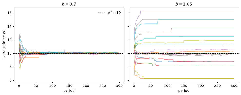
At \(b = 0.7\) every one of these runs settles at the rational expectations price.
At \(b = 1.05\) only a few runs end near it.
The others are pushed away in the first few periods, while the population is still diverse.
They then stall, apart from occasional jumps, at a forecast that is wrong in the same direction every period.
The T-map of One recursion, many learners explains the direction.
A population whose average forecast is \(\bar\beta\) induces the price \(T(\bar\beta) = a + b\bar\beta\) on average, and selection and election favor forecasts near the realized price.
Since \(T(\bar\beta) - \bar\beta = (b - 1)(\bar\beta - p^*)\), the favored forecasts lie on the side of \(p^*\) when \(b < 1\) and on the far side when \(b > 1\).
The genetic algorithm lies outside the theory of stochastic approximation, but here it moves in the direction that the theory’s mean dynamics would predict.
Why does it stall rather than run off to the edge of \([0, 20]\)?
Because \(b\) is close to 1, the push is weak: a population 1.5 away from \(p^*\) makes systematic forecast errors of only \(0.05 \times 1.5 = 0.075\) a period, less than the noise.
And once the strings are nearly identical, crossover creates nothing new, and many small moves of the forecast require several bits to flip at once (a “Hamming cliff” of binary encoding), so the population can freeze.
So the experiment agrees with the book in a weak sense.
When \(b > 1\) the population ends near the rational expectations price only in runs that happened to stall near it.
The equilibrium does not attract it, and it does not attract least squares either, which diverges when \(b > 1\), though very slowly when \(b\) is this close to 1 (Least Squares Learning in Self-Referential Models).
The election operator matters even when \(b = 0.7\).
Remove it, and the population keeps its children however badly they forecast, and it settles much less tightly on \(p^*\): as in Exchange Rate Indeterminacy, Learning, and Experiments, election is what lets a genetic population learn, by making it homogeneous.
Exercise 94.5
Extend the two-link chain of The bucket brigade by giving the system a choice at the first stage.
A myopic rule \(m\) collects \(r_m = 1\) at once and ends the episode.
The setup rule \(s\) collects nothing but moves the system to a second stage, where the payoff rule \(p\) collects \(R\).
To separate the accounting from the auction, choose \(m\) or \(s\) at random with equal probability in every episode, and use the averaging accounting with \(b = 0.1\).
Suppose there are no backward payments: the payoff rule’s bid is paid to no one. What happens to the setup rule’s strength?
With the payoff rule paying its bid to the setup rule, find the stationary strengths of \(m\) and \(s\), and the smallest ratio \(R/r_m\) at which an argmax auction would choose the setup rule. Check your answer by simulation.
Repeat part 2 with Holland’s cumulative balances. Which accounting is more patient?
Solution
Here is the chain with a choice at its first stage.
def two_stage(R, r_m=1.0, b=0.1, T=20_000, accounting='average', backward=True, seed=0):
    "Strengths of [myopic, setup, payoff] when the first-stage rule is chosen at random."
    rng = np.random.default_rng(seed)
    S, τ = np.zeros(3), np.zeros(3)
    for _ in range(T):
        if rng.random() < 0.5:
            acts = [(0, r_m)]                                  # myopic: paid at once
        else:
            acts = [(1, b * S[2] if backward else 0.0),        # setup: paid the next bid
                    (2, R)]                                    # payoff: paid by the world
        for k, receipts in acts:
            τ[k] += 1
            if accounting == 'average':
                S[k] += (receipts - (1 + b) * S[k]) / τ[k]
            else:
                S[k] += receipts - b * S[k]
    return S

b = 0.1
print(f"predicted threshold R / r_m = (1 + b) / b = {(1 + b) / b:.1f}\n")
for R in (5.0, 10.0, 12.0, 20.0):
    rows = {'no backward payment': two_stage(R, backward=False),
            'average': two_stage(R),
            'balance': two_stage(R, accounting='balance')}
    for name, S in rows.items():
        winner = 'setup' if S[1] > S[0] else 'myopic'
        print(f"R = {R:>4}, {name:>19}: S_m = {S[0]:7.3f}, S_s = {S[1]:7.3f}  -> {winner}")
    print()
predicted threshold R / r_m = (1 + b) / b = 11.0

R =  5.0, no backward payment: S_m =   0.909, S_s =   0.000  -> myopic
R =  5.0,             average: S_m =   0.909, S_s =   0.413  -> myopic
R =  5.0,             balance: S_m =  10.000, S_s =  50.000  -> setup
R = 10.0, no backward payment: S_m =   0.909, S_s =   0.000  -> myopic
R = 10.0,             average: S_m =   0.909, S_s =   0.826  -> myopic
R = 10.0,             balance: S_m =  10.000, S_s = 100.000  -> setup

R = 12.0, no backward payment: S_m =   0.909, S_s =   0.000  -> myopic
R = 12.0,             average: S_m =   0.909, S_s =   0.992  -> setup
R = 12.0,             balance: S_m =  10.000, S_s = 120.000  -> setup
R = 20.0, no backward payment: S_m =   0.909, S_s =   0.000  -> myopic
R = 20.0,             average: S_m =   0.909, S_s =   1.653  -> setup
R = 20.0,             balance: S_m =  10.000, S_s = 200.000  -> setup
Part 1. Without backward payments the setup rule’s receipts are always zero, so its strength never rises above zero, however large \(R\) is.
No auction based on strength would ever choose it.
Part 2. With averaging, the stationary strengths solve \((1+b)S_m = r_m\), \((1+b)S_p = R\) and \((1+b)S_s = b S_p\), so
The setup rule wins exactly when \(R / r_m > (1 + b)/b = 11\).
The simulation confirms it: the setup rule loses at \(R = 10\) and wins at \(R = 12\).
Part 3. With cumulative balances, \(S_m = r_m/b\) and \(S_s = S_p = R/b\), so the setup rule wins whenever \(R > r_m\).
Holland’s accounting is patient; the averaging accounting is very impatient.
A classifier system that averages its strengths with \(b = 0.1\) prefers 1 now to 10 one step later.
The bucket brigade’s discount factor shows how the same arithmetic, applied to the chain that links trading to consuming, makes the agents of Money as a Medium of Exchange among Artificially Intelligent Agents effectively very impatient.