109. The Lost Conquest: Fed Policy in the 2020s#
109.1. Overview#
The previous lecture, Drifts and Volatilities after 2000, carried the drifting-coefficients evidence of Cogley and Sargent [2005] past 2000: it asked how the reduced-form dynamics of inflation, and the volatilities of the shocks hitting them, moved in the decades after the Conquest was written.
This final lecture of the suite takes the policy maker’s point of view instead.
It follows Sargent and Williams [2025], who impute drifting beliefs to the Federal Reserve and ask what policy those beliefs recommended during the inflation of the 2020s.
Their artificial Fed is built from tools that earlier lectures developed:
the anticipated-utility assumption of Kreps [1998], met in Adaptive Learning and Escape Dynamics;
a drifting-coefficients model estimated by constant-gain recursive least squares, the constant-gain special case of the Kalman filter of Priors, Escapes, and Learning Cycles.
The puzzle is a live one.
After the COVID-19 pandemic, U.S. inflation surged to its highest rate since the early 1980s, the episode at the end of the post-1999 data in The Rise and Fall of U.S. Inflation.
That lecture plots CPI inflation; here, following the paper, we use the price index for personal consumption expenditures (PCE), the Fed’s preferred measure.
Yet for more than a year the Federal Reserve did not respond.
It first raised its policy rate in March 2022 and began to tighten in earnest only in the second quarter of 2022, with inflation already at its peak.
Why was the Fed so slow?
Sargent and Williams [2025] build an artificial Fed that, each quarter,
re-estimates a drifting-coefficients Phillips curve by constant-gain recursive least squares, and
solves a linear-quadratic Phelps problem, treating its latest estimates as if they would hold forever, to set its interest-rate instrument.
Control engineers call this model predictive control.
It is the estimate-then-optimize loop that drove the learning government of Adaptive Learning and Escape Dynamics, but now the instrument is the policy rate and the beliefs concern the persistence of inflation and the slope of the Phillips curve.
Three elements shape the artificial Fed’s decisions:
Declining inflation persistence. The Fed had learned that inflation shocks fade faster than they used to, so the surge looked transitory.
A flatter Phillips curve. The Fed had learned that inflation responds weakly to slack, so disinflation looked costly.
Real-time mismeasurement of the output gap. In real time the Fed perceived more slack than the revised data now show.
We reproduce all three from public data.
The main finding, which is also the paper’s, fits in one sentence:
drifting beliefs make the response muted; real-time mismeasurement makes it late.
With today’s revised data, the artificial Fed responds to the 2021 surge mildly, but earlier than the actual Fed did.
Only with the output gap that the Fed saw in real time does its response arrive at about the time the Fed’s did.
The last part of the lecture is our own extension.
It asks where the benign beliefs came from: can aggressive past policy make inflation look transitory and the Phillips curve look flat?
We compute the self-confirming fixed point of that loop and find that, unlike the government of Escaping Nash Inflation, this Fed has no escape route.
Note
Readers arriving from the Bounded Rationality suite will find \(\gamma\) in its usual role as the learning gain.
There the beliefs are called \(\alpha\) (Notation across the series, A government learning the Phillips curve); here they are \(\theta_t\).
Let’s import what we need:
import time
import matplotlib.pyplot as plt
import numpy as np
import pandas as pd
from scipy.linalg import solve_discrete_are
from scipy.optimize import brentq
109.2. The three elements#
The first two elements are among the most documented facts in modern macroeconomics.
Declining persistence. From the 1970s into the 1980s inflation was highly persistent: a shock raised inflation for years.
Cogley and Sargent [2001] and Cogley and Sargent [2005] documented the decline in inflation persistence during the Volcker–Greenspan conquest.
Drifts and Volatilities reproduces their evidence (Inflation persistence), and Drifts and Volatilities after 2000 carries it past 2000 (Core inflation, the natural rate, and persistence).
Stock and Watson [2007] found that the permanent component of inflation shrank in the 1980s and 1990s.
Benati and Surico [2008] and Carlstrom et al. [2009] linked the decline in persistence to more aggressive monetary policy, a link we take up in From policy to measured beliefs.
Pivetta and Reis [2007] cautioned that part of the apparent decline may reflect smaller shocks rather than a structural break; that is the distinction between drifting coefficients and drifting volatilities that Drifts and Volatilities draws.
Former Fed Chair Janet Yellen summarized the evidence in 2019: “the slope of the Phillips curve … has diminished very significantly since the 1960s … And second, inflation has become much less persistent, because the impact of lagged inflation on current inflation has declined considerably.”
A flatter Phillips curve. Since the 1990s, estimates of the Phillips curve’s slope have trended toward zero; the “missing disinflation” after the Great Recession is the leading example.
Policy makers knew what this implied.
Bernanke [2022] (p. 220) writes: “A flat Phillips curve means that inflation is a less reliable indicator of economic overheating. Should inflation get too high, the costs, in terms of unemployment, of bringing inflation back down to target could be higher than in the past.”
Notice that a flat Phillips curve points policy in opposite directions here and in the Conquest.
In the Lucas-style models of Sargent [1999], a flatter curve means that surprise inflation does less to real activity, so the Phelps problem recommends lower inflation.
The induction hypothesis of Adaptive Expectations and the Phelps Problem (Testing the natural-rate hypothesis), under which inflation has no long-run real effect, is the limiting case, and it is how the Conquest’s adaptive government brings inflation down.
In the statistical model of the 2020s, the Fed controls inflation by moving the output gap.
There a flatter curve means a higher sacrifice ratio (The sacrifice ratio): each point of disinflation costs more output, so the Phelps problem counsels patience (Sargent and Williams [2025], footnote 5).
Real-time uncertainty. The third element, emphasized by Orphanides [2001], is that the output gap is badly mismeasured in real time, especially at business-cycle turning points.
Through 2020–2023 the real-time gap was persistently below the later revised measure, so the Fed perceived more slack than there was.
We measure this in Real-time data and the delay.
109.3. The Fed’s drifting-coefficients beliefs#
We give the artificial Fed a backward-looking Phillips curve with drifting coefficients,
where \(\pi_t\) is four-quarter PCE inflation, \(x_t\) is the CBO output gap, \(\rho_t\) is the perceived persistence, and \(\kappa_t\) is the perceived slope.
\(\rho_t\) plays the role that the sum of the coefficients on lagged inflation plays in the Conquest’s Phelps problems (Testing the natural-rate hypothesis; Sargent and Williams [2025], footnote 11).
The Fed updates \(\theta_t = (\alpha_{0,t}, \rho_t, \kappa_t)^\top\) by constant-gain recursive least squares,
with regressors \(X_t = (1, \pi_{t-1}, x_t)^\top\) and moment matrix \(M_t\).
The estimate \(\theta_t\) uses data through quarter \(t\), and it is what the Fed brings to its decision in quarter \(t\).
The moment matrix is updated before the coefficients, the timing of Evans and Honkapohja [2001].
The paper’s display writes the lagged matrix \(M_{t-1}\) in the coefficient update.
The two timings differ by terms of order \(\gamma^2\) unless the regressors move far outside their past range.
In 2022 they did, and the timing then changes the recommendations noticeably, so it is worth saying which one the code uses.
The gain \(\gamma = 0.03\) is the paper’s choice for quarterly data; it discounts past observations so that the estimates can track drift.
Constant-gain least squares is the special case of the Kalman filter of Priors, Escapes, and Learning Cycles (see also A First Look at the Kalman Filter) that Sargent and Williams [2005] obtain with a particular prior about how the coefficients drift.
Which gain best rationalizes the Fed’s decisions is a version of Chung’s problem, which we pose in Exercise 109.4.
We read the PCE price index, real GDP, CBO potential output, and the federal funds rate directly from FRED.
If FRED lacks an isolated month, as happened for some series around the federal government shutdown of October 2025, the code fills it by linear interpolation and says so.
FRED = 'https://fred.stlouisfed.org/graph/fredgraph.csv?id='

def fred(series_id):
    "Read one series directly from FRED."
    s = pd.read_csv(FRED + series_id, index_col=0, parse_dates=True).iloc[:, 0]
    s.index.name = None
    return pd.to_numeric(s, errors='coerce')      # FRED marks gaps with '.'

def quarterly_mean(monthly):
    "Quarterly averages of a monthly series, filling isolated missing months."
    monthly = monthly.asfreq('MS')
    missing = monthly.index[monthly.isna()]
    if len(missing) > 0:
        print(f"{monthly.name}: interpolating",
              [f"{d:%Y-%m}" for d in missing])
    filled = monthly.interpolate(limit=1, limit_area='inside')
    q = filled.resample('QS')
    return q.mean()[q.count() == 3]                # complete quarters only

def qtr(date):
    "Label a date by its quarter, e.g. 2022Q2."
    return f"{date.year}Q{date.quarter}"

pce = quarterly_mean(fred('PCEPI'))
fedfunds = quarterly_mean(fred('FEDFUNDS'))
gdp, potential = fred('GDPC1'), fred('GDPPOT')     # real GDP, CBO potential

inflation = 100 * (pce / pce.shift(4) - 1)          # four-quarter PCE inflation
gap = 100 * (gdp / potential - 1)                   # output gap, percent

data = pd.concat([inflation.rename('pi'), gap.rename('x'),
                  fedfunds.rename('i')], axis=1, sort=True).dropna().loc['1960':]
print(f"sample: {qtr(data.index[0])} to {qtr(data.index[-1])}, "
      f"{len(data)} quarters")

peak = data['pi']['2020':].idxmax()
higher = data['pi'][:peak].iloc[:-1]
last_higher = higher[higher > data['pi'][peak]].index[-1]
print(f"PCE inflation peaked at {data['pi'][peak]:.2f}% in {qtr(peak)}, "
      f"the highest since {qtr(last_higher)}")
sample: 1960Q1 to 2026Q3, 267 quarters
PCE inflation peaked at 6.88% in 2022Q2, the highest since 1981Q4
Following the paper, we freeze beliefs during 2020 and 2021, setting the gain to zero, because the pandemic observations were extreme outliers that would otherwise whipsaw the estimates; updating resumes in 2022.
The freeze is not innocuous.
The 2020 quarters are the true outliers, but it is the freeze of 2021 that drives the results below.
If the Fed had learned from the 2021 data, its perceived Phillips curve would have steepened and its recommended rate would have jumped to several percent by the end of 2021 (Exercise 109.3).
Setting the gain to zero in 2021 is itself the judgment that the 2021 surge was transitory.
We start the recursion at \(\theta = (0.5, 0.9, 0.05)\) rather than at the paper’s 1949–1959 presample regression; the belief paths after the mid-1980s hardly depend on this choice.
We compute the beliefs once and reuse them below.
def estimate_beliefs(data, γ=0.03, freeze=(2020, 2021)):
    "Constant-gain RLS for the drifting Phillips curve: paths of α₀, ρ, κ."
    π, x = data['pi'].values, data['x'].values
    θ = np.array([0.5, 0.9, 0.05])            # [intercept, persistence, slope]
    M = np.diag([1.0, 10.0, 5.0])             # moment matrix
    rows = []
    for t in range(1, len(data)):
        γ_t = 0.0 if data.index[t].year in freeze else γ
        X = np.array([1.0, π[t - 1], x[t]])
        M = M + γ_t * (np.outer(X, X) - M)                     # M_t first,
        θ = θ + γ_t * np.linalg.solve(M, X * (π[t] - X @ θ))   # then θ_t
        rows.append(θ)
    return pd.DataFrame(rows, index=data.index[1:],
                        columns=['alpha0', 'rho', 'kappa'])

beliefs = estimate_beliefs(data)
Here are the perceived persistence and slope.
fig, axes = plt.subplots(2, 1, figsize=(10, 6), sharex=True)
axes[0].plot(beliefs['rho'])
axes[0].axhline(1, color='k', lw=0.5, ls=':')
axes[0].set_ylabel(r'persistence $\rho_t$')

axes[1].plot(beliefs['kappa'], color='C1')
axes[1].axhline(0, color='k', lw=0.5, ls=':')
axes[1].set_ylabel(r'slope $\kappa_t$')
axes[1].set_xlabel('year')

plt.tight_layout()
plt.show()

ρ, κ = beliefs['rho'], beliefs['kappa']
after85 = ρ['1985':]
print(f"ρ_t over 1985-2001: mean {ρ['1985':'2001'].mean():.3f}, "
      f"range {ρ['1985':'2001'].min():.3f} to {ρ['1985':'2001'].max():.3f}")
print(f"first quarter after 1985 with ρ_t < 0.96: "
      f"{qtr(after85[after85 < 0.96].index[0])}")
print(f"trough of ρ_t: {ρ.min():.3f} in {qtr(ρ.idxmin())}")
print(f"κ_t: {κ['1980':'1984'].mean():.3f} (1980-84 average), "
      f"{κ['2009':'2009'].max():.3f} (2009 peak), "
      f"{κ['2019-10-01']:.3f} (2019Q4)")
print(f"2019Q4: ρ = {ρ['2019-10-01']:.3f};   2022Q2: ρ = {ρ['2022-04-01']:.3f}")
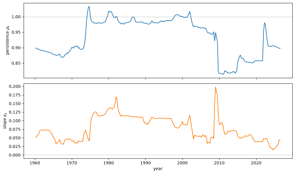
Fig. 109.1 The Fed’s perceived inflation persistence and Phillips curve slope#
ρ_t over 1985-2001: mean 0.989, range 0.976 to 1.010
first quarter after 1985 with ρ_t < 0.96: 2006Q3
trough of ρ_t: 0.814 in 2011Q1
κ_t: 0.131 (1980-84 average), 0.198 (2009 peak), 0.039 (2019Q4)
2019Q4: ρ = 0.858;   2022Q2: ρ = 0.981
Perceived persistence \(\rho_t\) jumps in the mid-1970s and then stays close to one for a quarter of a century, through 2001.
It drifts down only slowly in the 2000s and falls steeply after the 2008 recession, to a trough in 2011.
Sargent and Williams [2025] describe a decline after the mid-1980s “with an especially precipitous fall following the 2008 recession”; in this replication the decline is mainly that post-2008 fall.
When updating resumes in 2022, \(\rho_t\) jumps back toward one, just as the Fed abandoned the “transitory” characterization and began to tighten.
Perceived slope \(\kappa_t\) declines from its early-1980s level, spikes during the 2008–2009 recession, when the economy briefly experienced deflation, and is lower still by 2019: the Phillips curve flattens.
A word on the scale of \(\rho_t\).
Because \(\pi_t\) is a four-quarter rate, consecutive observations share three quarters of data.
Even if quarterly inflation were serially uncorrelated, a regression of \(\pi_t\) on \(\pi_{t-1}\) would give a coefficient near \(0.75\) (Exercise 109.5).
Against that floor, the 2019 value of \(\rho_t\) means less persistent, not transitory:
ρ_2019 = ρ['2019-10-01']
print(f"half-life of an inflation shock at ρ = {ρ_2019:.3f}: "
      f"{np.log(0.5) / np.log(ρ_2019):.1f} quarters")
half-life of an inflation shock at ρ = 0.858: 4.5 quarters
With quarterly annualized inflation, which has no overlap, the same algorithm finds persistence falling earlier and much further.
That measure is closer in spirit to the one in Drifts and Volatilities; Exercise 109.5 reconciles the two.
Still, by 2019 the Fed’s model said that inflation was less persistent than it used to be and only weakly linked to slack.
Fed into a Phelps problem, these beliefs counsel patience.
109.4. The Fed’s Phelps problem#
Each quarter the Fed sets its policy rate by solving a linear-quadratic Phelps problem, treating its current estimates as if they will hold forever.
That is the anticipated-utility assumption of Kreps [1998] that we met in Adaptive Learning and Escape Dynamics.
The belief Phillips curve (109.1) is paired with an IS curve
whose coefficients are estimated once, by OLS over the whole sample.
Together they give linear dynamics for the state \(s_t = (1, \pi_t, x_t, i_{t-1})^\top\),
whose matrices depend on the time-\(t\) beliefs.
The Fed minimizes
where \(\pi^* = 2\) is the target and the last term penalizes abrupt rate changes.
We use the paper’s parameter values: \(\beta = 0.95\), \(\lambda_x = 0.2\), and \(\eta = 0.5\).
The paper says these values were “loosely tuned to provide a reasonable match to the observed policy outcomes.”
Writing the period loss as \(s^\top Q s + 2 s^\top N i + R\, i^2\) with \(R = \eta\) turns this into a discounted linear-quadratic regulator with a cross term (LQ Control: Foundations).
The matrix \(P_t\) of the expected discounted loss \(s^\top P_t s\) (plus a constant) solves the discounted Riccati equation
and the decision rule is \(i_t = -F_t s_t\) with \(F_t = (R + \beta B^\top P_t B)^{-1}(\beta B^\top P_t A + N^\top)\).
Written out, the rule is a smoothed Taylor rule,
whose coefficients move as beliefs move.
scipy.linalg.solve_discrete_are solves the undiscounted version of (109.4).
Passing \(\sqrt\beta A\) and \(\sqrt\beta B\) absorbs the discount factor.
The cross term then enters unscaled, as s=N, because \(\beta A^\top P B + N = (\sqrt\beta A)^\top P (\sqrt\beta B) + N\).
Following the paper (Sargent and Williams [2025], section 3.3), we impose the zero lower bound only ex post, \(i^{\rm opt}_t = \max\{-F_t s_t, 0\}\).
The Fed’s Phelps problem does not anticipate that the bound might bind.
# IS curve, estimated once by OLS over the full sample
π_d, x_d, i_d = data['pi'].values, data['x'].values, data['i'].values
n = len(data)
Z_is = np.column_stack([np.ones(n - 1), x_d[:-1], i_d[:-1] - π_d[:-1]])
b0, b1, g = np.linalg.lstsq(Z_is, x_d[1:], rcond=None)[0]
print(f"IS curve: b0 = {b0:.3f}, b1 = {b1:.3f}, g = {g:.4f}; "
      f"long-run effect of the real rate g/(1-b1) = {g / (1 - b1):.2f}")

β, π_star, λ_x, η = 0.95, 2.0, 0.2, 0.5

def phelps_rule(θ, η=η):
    "Coefficients (ϕ₀, ϕ_π, ϕ_x, ϕ_i) of the Phelps rule i = -F s under beliefs θ."
    α0, ρ, κ = θ
    A = np.array([[1, 0, 0, 0],
                  [α0 + κ * b0, ρ - κ * g, κ * b1, 0],
                  [b0, -g, b1, 0],
                  [0, 0, 0, 0]], float)
    B = np.array([[0], [κ * g], [g], [1]], float)
    c_π = np.array([-π_star, 1, 0, 0.])       # π − π*
    c_x = np.array([0, 0, 1, 0.])             # x
    e_i = np.array([0, 0, 0, 1.])             # i_{t-1}
    Q = np.outer(c_π, c_π) + λ_x * np.outer(c_x, c_x) + η * np.outer(e_i, e_i)
    N = (-η * e_i).reshape(4, 1)
    R = np.array([[η]])
    # √β absorbs discounting in A and B; the cross term N enters unscaled
    P = solve_discrete_are(np.sqrt(β) * A, np.sqrt(β) * B, Q, R, s=N)
    F = np.linalg.solve(R + β * B.T @ P @ B, β * B.T @ P @ A + N.T)
    return -F.ravel()

def phelps_rules(beliefs, η=η):
    "The Phelps rule at every date, given a path of beliefs."
    return pd.DataFrame([phelps_rule(θ, η) for θ in beliefs.values],
                        index=beliefs.index,
                        columns=['φ_0', 'φ_π', 'φ_x', 'φ_i'])

def recommended_rate(data, rules):
    "Recommended rate max(-F_t s_t, 0): the zero lower bound imposed ex post."
    π, x, i = data['pi'].values, data['x'].values, data['i'].values
    s = np.column_stack([np.ones(len(data) - 1), π[1:], x[1:], i[:-1]])
    return pd.Series(np.maximum((rules.values * s).sum(axis=1), 0.0),
                     index=rules.index)

rules = phelps_rules(beliefs)
optimal = recommended_rate(data, rules)
IS curve: b0 = 0.013, b1 = 0.907, g = -0.0220; long-run effect of the real rate g/(1-b1) = -0.24
The estimated interest sensitivity \(g\) is small.
Policy endogeneity, which we meet again in From policy to measured beliefs, is one reason a regression can understate how much interest rates matter: a Fed that leans against expected booms weakens the correlation between the real rate and subsequent output.
fig, ax = plt.subplots(figsize=(10, 4.5))
window = slice('1991', None)
ax.plot(optimal[window], 'C0', label="Phelps problem's recommended rate")
ax.plot(data['i'][window], 'C3', lw=1, label='actual federal funds rate')
ax.set_xlabel('year')
ax.set_ylabel('percent')
ax.legend()
plt.show()

def fit(rate, start='1991'):
    "Correlation and root mean squared error against the actual funds rate."
    r = rate[start:]
    actual = data['i'][r.index]
    return np.corrcoef(r, actual)[0, 1], np.sqrt(((r - actual)**2).mean())

no_change = data['i'].shift(1).dropna()               # i_t = i_{t-1}
for name, rate in [('Phelps rule', optimal), ('no-change rule', no_change)]:
    c, rmse = fit(rate)
    print(f"{name:>15}: correlation {c:.3f}, RMSE {rmse:.2f} "
          f"(1991-{data.index[-1].year})")
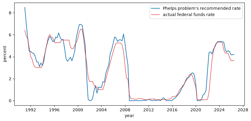
Fig. 109.2 The belief-driven Phelps rule against the actual federal funds rate#
    Phelps rule: correlation 0.944, RMSE 0.79 (1991-2026)
 no-change rule: correlation 0.979, RMSE 0.45 (1991-2026)
The subjectively optimal rate tracks the level and turning points of actual policy over three decades: the mid-1990s tightening, the 2001 easing, the zero-bound era after 2008, and the normalization that began in 2015.
It misses some episodes, falling well below the actual rate in 1998 and again in 2002.
The correlation needs a benchmark.
Because the recommendation conditions on the actual lagged rate \(i_{t-1}\), a naive rule that simply sets \(i_t = i_{t-1}\) does better on both measures, as the output shows.
The paper makes the same point about one-step-ahead fit.
What the Phelps rule offers is not a better forecast of the funds rate but an interpretation of it, in terms of beliefs and a loss function.
Now look at 2021.
Beliefs are frozen, but the state is not: as inflation and the output gap rise, the rule recommends a rising rate.
print(pd.DataFrame({'Phelps rule': optimal, 'actual': data['i']})
        .loc['2021':'2022'].rename(index=qtr).round(2).T.to_string())
             2021Q1  2021Q2  2021Q3  2021Q4  2022Q1  2022Q2  2022Q3  2022Q4
Phelps rule    0.13    0.53    0.62    0.96    2.76    4.38    4.44    4.25
actual         0.08    0.07    0.09    0.08    0.12    0.77    2.19    3.65
With today’s revised data, the artificial Fed starts raising its rate in 2021 and is well ahead of the actual Fed in early 2022.
So with current-vintage data the drifting-beliefs model leads the Fed rather than mirroring it, as the paper also finds when it uses revised data (Sargent and Williams [2025], section 3.5).
Drifting beliefs make the recommended response mild, but they do not make it late.
We return to the delay in Real-time data and the delay.
109.4.1. How the rule drifted#
The paper’s Figure 8 shows the mechanism directly: the coefficients of the Phelps rule, and the long-run response of the policy rate to inflation, \(\phi_{\pi,t}/(1-\phi_{i,t})\).
We compute them with today’s data; the paper’s figure uses real-time data.
A long-run response above one is the Taylor principle.
long_run = rules['φ_π'] / (1 - rules['φ_i'])

fig, axes = plt.subplots(3, 1, figsize=(10, 8), sharex=True)
axes[0].plot(rules['φ_π'], label=r'$\phi_{\pi,t}$')
axes[0].plot(rules['φ_x'], label=r'$\phi_{x,t}$')
axes[0].legend()
axes[0].set_ylabel('response')
axes[1].plot(rules['φ_i'], color='C2')
axes[1].set_ylabel(r'smoothing $\phi_{i,t}$')
axes[2].plot(long_run, color='C3')
axes[2].axhline(1, color='k', lw=0.5, ls=':')
axes[2].set_ylabel(r'$\phi_{\pi,t}/(1-\phi_{i,t})$')
axes[2].set_xlabel('year')
plt.tight_layout()
plt.show()

for date in ['2000-01-01', '2019-10-01']:
    print(f"long-run inflation response in {qtr(pd.Timestamp(date))}: "
          f"{long_run[date]:.2f}")
peak_lr = long_run['2021':'2023'].idxmax()
print(f"peak in 2021-2023: {long_run[peak_lr]:.2f} in {qtr(peak_lr)}")
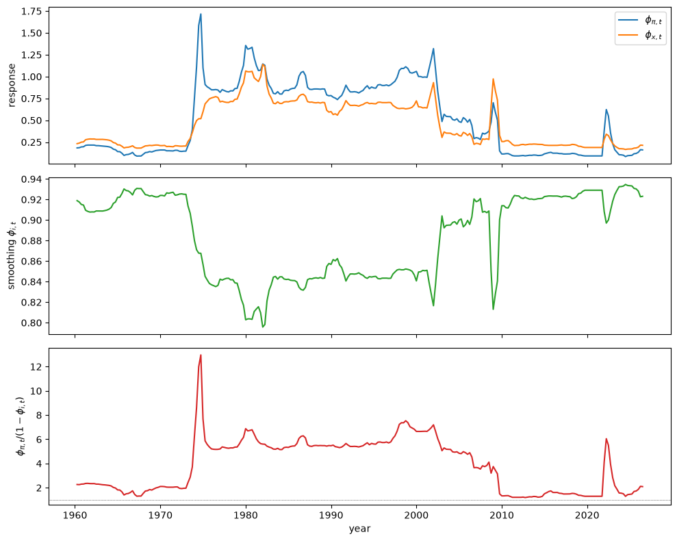
Fig. 109.3 Coefficients of the Phelps rule and its long-run response to inflation#
long-run inflation response in 2000Q1: 6.65
long-run inflation response in 2019Q4: 1.30
peak in 2021-2023: 6.05 in 2022Q2
As persistence and slope drifted down, the rule’s long-run response to inflation fell from well above one in 2000 to just above one by 2019, while interest-rate smoothing rose.
The 2019 rule barely satisfied the Taylor principle.
When updating resumed in 2022 and \(\rho_t\) jumped, the long-run response jumped with it, before falling back as inflation receded.
Part of the 2022 tightening in Fig. 109.2 therefore comes from a change in the rule itself, not only from the rise in inflation and the gap.
109.5. Why the Fed was slow: a counterfactual#
To isolate the role of the drifting beliefs, we recompute the Phelps recommendations holding beliefs fixed at their values in the first quarter of 2000.
θ_2000 = beliefs.loc['2000-01-01'].values
print(f"beliefs in 2000Q1: α₀ = {θ_2000[0]:.3f}, ρ = {θ_2000[1]:.3f}, "
      f"κ = {θ_2000[2]:.3f}")
beliefs in 2000Q1: α₀ = -0.025, ρ = 1.001, κ = 0.097
In 2000 the Fed’s model had a unit root: \(\rho \approx 1\), so inflation shocks were perceived as permanent.
Its perceived slope was more than twice the 2019 value.
rules_2000 = pd.DataFrame(np.tile(phelps_rule(θ_2000), (len(beliefs), 1)),
                          index=beliefs.index, columns=rules.columns)
counterfactual = recommended_rate(data, rules_2000)

fig, ax = plt.subplots(figsize=(10, 4.5))
w = slice('2015', None)
ax.plot(optimal[w], 'C0', label='baseline (drifting beliefs)')
ax.plot(counterfactual[w], 'C1--', label='counterfactual (beliefs frozen at 2000)')
ax.plot(data['i'][w], 'C3', lw=1, alpha=0.7, label='actual funds rate')
ax.set_xlabel('year')
ax.set_ylabel('percent')
ax.legend()
plt.show()

print(f"counterfactual rate in 2021Q4: {counterfactual['2021-10-01']:.2f}%  "
      f"(actual {data['i']['2021-10-01']:.2f}%)")
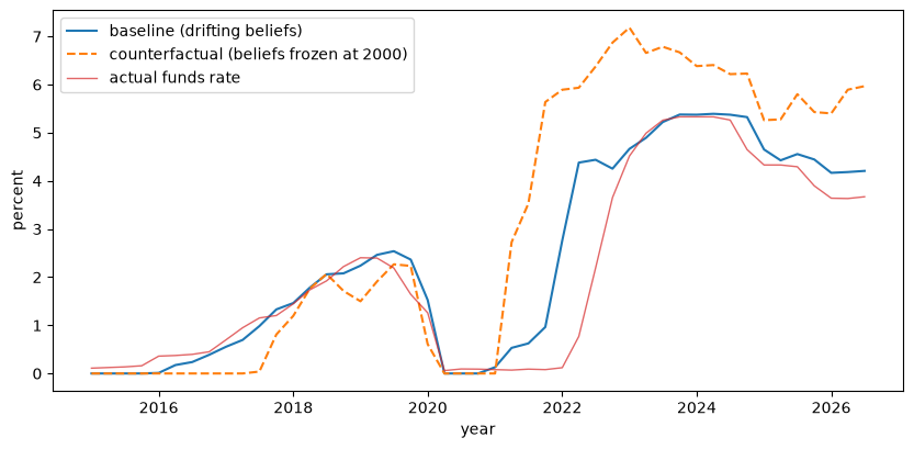
Fig. 109.4 Counterfactual: a Fed that had not updated its beliefs since 2000#
counterfactual rate in 2021Q4: 5.64% (actual 0.08%)
A Fed with year-2000 beliefs would have tightened immediately and sharply in 2021, driving the funds rate above 5% by the end of 2021, before the actual Fed had moved at all.
The objectives are the same in both paths; only the beliefs differ.
Perceiving inflation as less persistent and the Phillips curve as flatter, the Fed’s own Phelps problem told it to respond mildly.
This is the 2020s counterpart of Cogley and Sargent [2005]’s account of the 1970s.
There a Bayesian Fed ran a race among three Phelps problems, and the costly disinflation predicted by the worst-case Samuelson–Solow model made it gradual, even after the data favored a natural-rate model.
109.6. Real-time data and the delay#
The paper’s conclusion turns on the third element.
In its words, “Only by incorporating real-time uncertainty about the economy, which tends to be elevated during business cycle turning points, do we rationalize the observed delay in the policy response” (Sargent and Williams [2025], section 3.5).
We now rebuild the output gap that the Fed saw in real time.
ALFRED, the St. Louis Fed’s archive of past data vintages, keeps every vintage of real GDP (GDPC1) and of CBO potential output (GDPPOT).
For each quarter since 2019, we compute the gap from the two series as they stood 45 days after the quarter ended, by which time the advance GDP estimate is normally out.
Two kinds of quarters need care.
Some GDP releases were delayed by the federal government shutdown of late 2025. For any quarter missing from its 45-day vintage, we use the first later vintage that contains it.
In September 2023 the Bureau of Economic Analysis re-expressed real GDP in 2017 dollars, while CBO’s potential output stayed in 2012 dollars until early 2024. A gap computed from such a vintage compares series in different units. We detect this by the ratio of the two series before 2019 and skip vintages in which they are not on the same base.
ALFRED serves up to twelve series per request, so the code asks for six vintages of both series at a time, and the whole history takes only a few requests.
ALFRED = 'https://alfred.stlouisfed.org/graph/alfredgraph.csv'

def alfred_vintages(series, dates, per_request=6, tries=3):
    "Vintages of several series at several dates, a few requests in all."
    frames = []
    for j in range(0, len(dates), per_request):
        vd = [f"{d:%Y-%m-%d}" for d in dates[j:j + per_request]]
        url = (f"{ALFRED}?id={','.join(s for s in series for _ in vd)}"
               f"&vintage_date={','.join(vd * len(series))}")
        for attempt in range(tries):
            try:
                frames.append(pd.read_csv(url, index_col=0, parse_dates=True))
                break
            except Exception as err:
                if attempt == tries - 1:
                    raise RuntimeError(
                        "Could not download data vintages from ALFRED "
                        f"(alfred.stlouisfed.org): {err}. This section "
                        "needs internet access to ALFRED.") from err
                time.sleep(5)
    print(f"{len(frames)} requests to ALFRED")
    return pd.concat(frames, axis=1).apply(pd.to_numeric, errors='coerce')

def real_time_gap(quarters, lag_days=45):
    "Output gap for each quarter from the first suitable vintage after it ends."
    # ALFRED relabels a vintage date it treats as still in the future, as it
    # does with today's date for some hours after midnight in St. Louis
    latest = (pd.Timestamp.now(tz='America/Chicago').tz_localize(None).normalize()
              - pd.Timedelta(days=1))
    vintages = sorted({min(q + pd.offsets.QuarterEnd(0)
                           + pd.Timedelta(days=lag_days), latest)
                       for q in quarters})
    V = alfred_vintages(['GDPC1', 'GDPPOT'], vintages)
    base = slice('2015-01-01', '2018-10-01')        # a pre-pandemic window
    gap, late = {}, []
    for q in quarters:
        target = min(q + pd.offsets.QuarterEnd(0) + pd.Timedelta(days=lag_days),
                     latest)
        for v in vintages:
            if v <= q + pd.offsets.QuarterEnd(0):
                continue
            y, y_pot = V[f'GDPC1_{v:%Y%m%d}'], V[f'GDPPOT_{v:%Y%m%d}']
            if pd.isna(y.get(q)) or pd.isna(y_pot.get(q)):
                continue                                # not yet released
            if abs(np.log(y[base] / y_pot[base]).mean()) > 0.04:
                continue                                # different base years
            gap[q] = 100 * (y[q] / y_pot[q] - 1)
            if v != target:
                late.append(f"{qtr(q)} (vintage {v:%Y-%m-%d})")
            break
    print("quarters taken from a later vintage:", late)
    return pd.Series(gap)

x_real_time = real_time_gap(data.loc['2019':].index)
6 requests to ALFRED
quarters taken from a later vintage: ['2023Q3 (vintage 2024-02-14)', '2025Q3 (vintage 2026-02-14)', '2025Q4 (vintage 2026-05-15)']
Here is the real-time gap against the gap in today’s data.
x_now = data['x'][x_real_time.index]
fig, ax = plt.subplots(figsize=(10, 4.5))
ax.plot(x_now, 'C0', label="today's data")
ax.plot(x_real_time, 'C1--', marker='o', ms=3, label='real time (ALFRED)')
ax.axhline(0, color='k', lw=0.5, ls=':')
ax.set_xlabel('year')
ax.set_ylabel('percent of potential')
ax.legend()
plt.show()

diff = x_real_time - x_now
below = diff['2020':'2023'] < 0
print(f"real-time gap below today's gap in {below.sum()} of {len(below)} "
      f"quarters of 2020-2023; largest shortfall {-diff.min():.2f} pp "
      f"in {qtr(diff.idxmin())}")
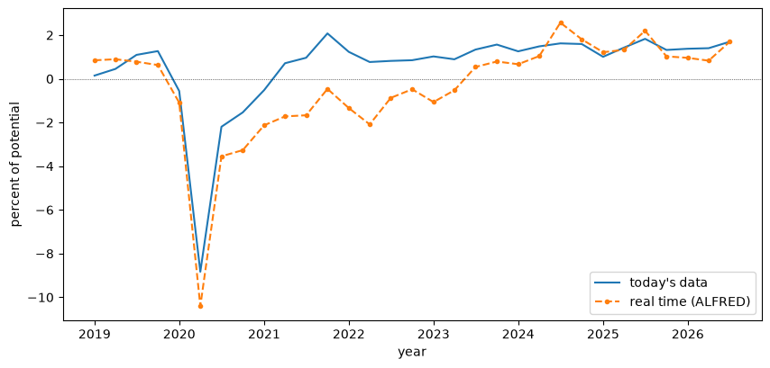
Fig. 109.5 The output gap in real time and in today’s data#
real-time gap below today's gap in 16 of 16 quarters of 2020-2023; largest shortfall 2.85 pp in 2022Q2
From 2020 through 2023 the real-time gap was below the revised gap in every quarter, by up to about three percentage points.
In real time, the 2021 boom looked like a slow recovery from a deep recession.
We now give the artificial Fed the real-time gap from 2019 on, re-estimate its beliefs, and recompute its recommendations, holding the IS curve fixed.
data_rt = data.copy()
data_rt.loc[x_real_time.index, 'x'] = x_real_time.values
beliefs_rt = estimate_beliefs(data_rt)
optimal_rt = recommended_rate(data_rt, phelps_rules(beliefs_rt))

fig, ax = plt.subplots(figsize=(10, 4.5))
w = slice('2019', None)
ax.plot(optimal[w], 'C0', label="Phelps rule, today's data")
ax.plot(optimal_rt[w], 'C1--', label='Phelps rule, real-time gap')
ax.plot(data['i'][w], 'C3', lw=1, label='actual funds rate')
ax.set_xlabel('year')
ax.set_ylabel('percent')
ax.legend()
plt.show()

table = pd.DataFrame({"today's data": optimal, 'real time': optimal_rt,
                      'actual': data['i']}).loc['2021':'2023-06']
print(table.rename(index=qtr).round(2).T.to_string())
print("\nmean rate in 2021:", table.loc['2021'].mean().round(2).to_dict())
for name in table:
    liftoff = table.index[table[name] > 0.5][0]
    print(f"first quarter above 0.5%, {name:>12}: {qtr(liftoff)}")
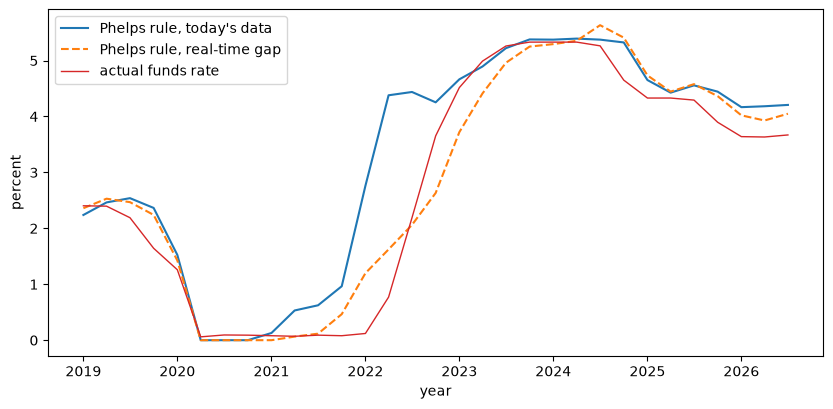
Fig. 109.6 Recommended rates with the revised and the real-time output gap#
              2021Q1  2021Q2  2021Q3  2021Q4  2022Q1  2022Q2  2022Q3  2022Q4  2023Q1  2023Q2
today's data    0.13    0.53    0.62    0.96    2.76    4.38    4.44    4.25    4.66    4.89
real time       0.00    0.06    0.12    0.47    1.20    1.62    2.06    2.63    3.72    4.41
actual          0.08    0.07    0.09    0.08    0.12    0.77    2.19    3.65    4.52    4.99

mean rate in 2021: {"today's data": 0.56, 'real time': 0.16, 'actual': 0.08}
first quarter above 0.5%, today's data: 2021Q2
first quarter above 0.5%,    real time: 2022Q1
first quarter above 0.5%,       actual: 2022Q2
With the gap that the Fed saw in real time, the recommended rate stays below half a percent through 2021.
It starts to rise at the turn of 2022, about when the Fed lifted off.
It runs ahead of the actual rate in the first half of 2022 and falls behind it from the third quarter on, as the Fed tightened in large steps.
That is the paper’s “slightly lagging” pattern.
With today’s data, by contrast, the rule lifts off about a year before the Fed did.
Putting the pieces together:
the counterfactual shows that drifting beliefs make the response muted: with its 2000 beliefs the Fed would have tightened fast and far;
this comparison shows that real-time mismeasurement makes it late: with drifting beliefs but accurate data, the Fed would have started tightening in 2021.
Both are needed to rationalize what the Fed did.
109.7. How beliefs shape the Phelps rule#
Why do lower perceived persistence and a flatter perceived slope make the rule less aggressive?
Sargent and Williams [2025] answer analytically, in their Appendix A, for a stripped-down version of the Phelps problem.
The Fed believes that
with \(|b_1| < 1\), \(\kappa > 0\), and \(g < 0\).
These are the paper’s equations (6) and (7), whose \(a_1\) and \(k\) are our \(\rho\) and \(\kappa\).
The Fed minimizes \(\mathbb{E} \sum_t \beta^t (\pi_t^2 + \lambda_x x_t^2)\), with no smoothing penalty, no intercepts, and a zero target.
Taking the real rate \(r_t = i_t - \pi_t\) as the control gives a regulator with state \((\pi_t, x_t)\) whose Riccati equation has a closed-form solution.
The optimal rule is \(i_t = \phi_\pi(\rho, \kappa)\, \pi_t + \phi_x x_t\) with
where
The paper proves two comparative statics.
Proposition 109.1 (Lower perceived persistence ⇒ less aggressive policy)
For any \(\beta \in (0,1)\), \(\lambda_x > 0\), \(\kappa > 0\), and \(g < 0\), the inflation coefficient \(\phi_\pi(\rho, \kappa)\) is strictly increasing in \(\rho \geq 0\).
Proposition 109.2 (Flatter perceived slope ⇒ less aggressive policy)
\(\partial \phi_\pi / \partial \kappa > 0\) whenever a sufficient condition (the paper’s inequality (11)) holds; it holds for small and moderate \(\kappa\).
Let’s verify both numerically, and check the closed form against solve_discrete_are along the way.
For the IS beliefs we use illustrative values, \(b_1 = 0.9\) and \(g = -0.5\).
\(b_1\) is close to the estimate above, but \(g\) is much larger in absolute value, so that \(\phi_\pi\) is of a familiar size.
Since \(\phi_\pi - 1\) is proportional to \(1/g\), the value of \(g\) does not affect the signs of the comparative statics.
def φ_π(ρ, κ, b1=0.9, g=-0.5, λ_x=0.2, β=0.95):
    "Closed-form inflation coefficient of the simplified Phelps rule."
    Δ = λ_x * (1 - β * ρ**2) - κ**2
    Z = (-Δ + np.sqrt(Δ**2 + 4 * λ_x * κ**2)) / 2
    return 1 - (ρ / (g * κ)) * Z / (Z + λ_x)

def φ_π_riccati(ρ, κ, b1=0.9, g=-0.5, λ_x=0.2, β=0.95, η_r=1e-9):
    "The same coefficient from solve_discrete_are, with control cost η_r r²."
    A = np.array([[ρ, κ * b1], [0, b1]])
    B = np.array([[κ * g], [g]])
    Q, R = np.diag([1, λ_x]), np.array([[η_r]])
    P = solve_discrete_are(np.sqrt(β) * A, np.sqrt(β) * B, Q, R)
    F = np.linalg.solve(R + β * B.T @ P @ B, β * B.T @ P @ A)
    return 1 - F[0, 0]

grid = [(ρ_, κ_) for ρ_ in np.linspace(0.05, 0.99, 12)
        for κ_ in np.linspace(0.01, 1.0, 12)]
gap_cf = max(abs(φ_π(*p) - φ_π_riccati(*p)) / φ_π(*p) for p in grid)
print(f"largest relative difference, closed form vs Riccati: {gap_cf:.1e}")
largest relative difference, closed form vs Riccati: 1.5e-08
The closed form checks out.
Now the two comparative statics.
ρ_grid = np.linspace(0, 0.999, 200)
κ_grid = np.linspace(0.005, 1.0, 400)

fig, axes = plt.subplots(1, 2, figsize=(11, 4))
for κ_ in [0.04, 0.1, 0.3]:
    axes[0].plot(ρ_grid, φ_π(ρ_grid, κ_), label=rf'$\kappa = {κ_}$')
axes[0].set_xlabel(r'perceived persistence $\rho$')
axes[0].set_ylabel(r'$\phi_\pi$')
axes[0].legend()

for ρ_ in [0.5, 0.86, 0.99]:
    axes[1].plot(κ_grid, φ_π(ρ_, κ_grid), label=rf'$\rho = {ρ_}$')
axes[1].set_xlabel(r'perceived slope $\kappa$')
axes[1].legend()
plt.tight_layout()
plt.show()

increasing = all(np.all(np.diff(φ_π(ρ_grid, κ_)) > 0)
                 for κ_ in [0.01, 0.04, 0.1, 0.3, 1.0, 3.0])
print("ϕ_π increasing in ρ for every κ tried:", increasing)
for ρ_ in [0.5, 0.86, 0.99]:
    κ_peak = κ_grid[np.argmax(φ_π(ρ_, κ_grid))]
    print(f"ρ = {ρ_}: ϕ_π increases in κ up to κ = {κ_peak:.3f}, then falls")
print(f"largest κ_t estimated in 2010-2019: {κ['2010':'2019'].max():.3f}")
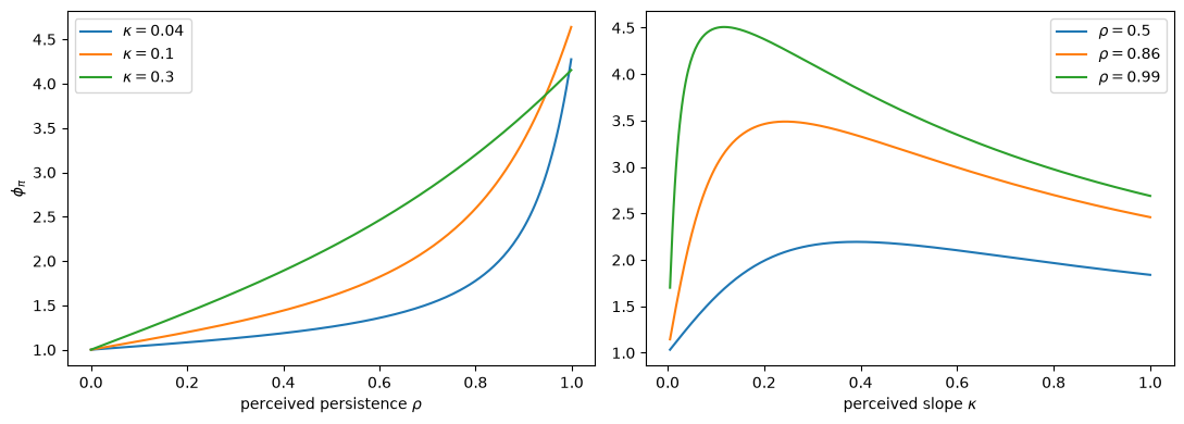
Fig. 109.7 The inflation coefficient of the simplified Phelps rule#
ϕ_π increasing in ρ for every κ tried: True
ρ = 0.5: ϕ_π increases in κ up to κ = 0.392, then falls
ρ = 0.86: ϕ_π increases in κ up to κ = 0.244, then falls
ρ = 0.99: ϕ_π increases in κ up to κ = 0.117, then falls
largest κ_t estimated in 2010-2019: 0.094
Persistence matters everywhere.
The higher \(\rho\), the more today’s inflation predicts future inflation, and the harder the Fed leans against it.
The slope matters too: a flatter curve makes each point of disinflation cost more output, so the Fed responds less.
That holds for small slopes, including all those the Fed estimated in the 2010s.
For large slopes the effect reverses, and the peak moves to smaller \(\kappa\) as \(\rho\) rises (Exercise 109.2).
So Proposition 109.2 should be read as a statement about small slopes.
Together, the two propositions explain the drift of the rule in Fig. 109.3: as \(\rho_t\) and \(\kappa_t\) fell, so did the rule’s response to inflation.
109.8. From policy to measured beliefs#
So far we have taken the Fed’s beliefs from the data.
Where did they come from?
In the extended abstract of their project, Sargent and Williams [2025] suggest that “the perceptions of the low persistence of inflation and a flat Phillips curve were based on the past Fed policy, which had reacted strongly to shocks and stabilized inflation.”
They frame the outcome as a self-confirming equilibrium in which the Fed is caught in a lack-of-experimentation trap.
This section is the lecture’s own extension of that idea; the January 2026 version of the paper does not contain it.
We put a small New Keynesian model on the table as nature’s model.
We compute what the Fed’s regression would measure under different policies, and then close the loop with the Phelps rule of the previous section.
In the terms of Koopmans [1947], the Fed’s drifting-coefficients model is a descriptive “Kepler stage” model.
Nature’s model, by contrast, is a “Newton stage” model whose parameters are invariant to the Fed’s rule.
109.8.1. Nature’s model#
Suppose that nature runs
where \(u_t\) is a cost-push shock and \(r_t\) a natural-rate (demand) shock.
The two shocks are IID and mutually uncorrelated, with standard deviations \(\sigma_u\) and \(\sigma_r\).
The first equation is the hybrid Phillips curve that arises when firms that cannot reset their prices index them to lagged inflation at rate \(\omega \in [0, 1]\).
Its weights on expected and lagged inflation sum to \((\beta_n + \omega)/(1 + \beta_n\omega) \leq 1\).
With this normalization the Taylor principle \(\phi > 1\) delivers a determinate equilibrium, which the code below checks by counting roots (Stability in Linear Rational Expectations Models; [Blanchard and Kahn, 1980]).
Nature’s discount factor \(\beta_n = 0.99\) is distinct from the Fed’s \(\beta = 0.95\).
We set \(\omega = 1\), a structural slope \(\kappa = 0.1\), and \(\sigma = 1\).
In the minimum-state-variable equilibrium, \(\mathbb{E}_t \pi_{t+1} = \lambda\, \pi_t\), and
Here \(\lambda\) is the stable root of the cubic
\(\psi = -\sigma\lambda(\phi - \lambda)/(1 - \lambda)\), and the impact coefficients \((a, b, c, d)\) are computed in the code.
\(\lambda\) is the coefficient of a univariate AR(1): it is what an econometrician who regressed inflation on its own lag would call persistence.
109.8.2. What the Fed measures#
The Fed’s regression (109.1) also contains \(x_t\).
Since \(x_t = \psi\, \pi_{t-1} + v_t\), with \(v_t = c\, u_t + d\, r_t\) uncorrelated with \(\pi_{t-1}\), its population coefficients are
So the Fed’s measured persistence \(\hat\rho\) is not \(\lambda\).
When only demand shocks hit (\(\sigma_u = 0\)), we can substitute \(\mathbb{E}_t\pi_{t+1} = \lambda\pi_t\) into the Phillips curve.
That gives the exact relation \(\pi_t = [\omega_b\, \pi_{t-1} + \kappa\, x_t]/(1 - \beta_f\lambda)\), so
The Fed recovers the structural lag weight and slope, each divided by \(1 - \beta_f\lambda(\phi)\), a factor that depends on policy.
That is the Lucas critique in one line.
A more aggressive rule lowers \(\lambda\), and with it both \(\hat\rho\) and \(\hat\kappa\): aggressive policy makes inflation look less persistent and the Phillips curve look flatter.
The persistence result is in the spirit of Benati and Surico [2008] and Carlstrom et al. [2009]; the slope result in this form is Bullard [2018]’s.
Cost-push shocks push \(\hat\kappa\) down further and can make it negative.
That is the identification problem stressed by McLeay and Tenreyro [2019]: when the Fed offsets cost-push shocks, high inflation coincides with a low output gap.
def nk_weights(ω, β_n=0.99):
    "Weights (β_f, ω_b) of the normalized hybrid Phillips curve."
    return β_n / (1 + β_n * ω), ω / (1 + β_n * ω)

def nk_roots(φ, ω=1.0, κ=0.1, σ=1.0, β_n=0.99):
    "Roots of the cubic whose stable root is λ."
    β_f, ω_b = nk_weights(ω, β_n)
    return np.roots([β_f, -(1 + β_f + κ * σ), 1 + ω_b + κ * σ * φ, -ω_b])

def fed_regression(φ, ω=1.0, κ=0.1, σ=1.0, β_n=0.99, σ_u=0.0, σ_r=1.0):
    "λ, and the Fed's population estimates (ρ̂, κ̂), when nature's rule is φ."
    β_f, ω_b = nk_weights(ω, β_n)
    roots = nk_roots(φ, ω, κ, σ, β_n)
    λ = roots[np.abs(roots) < 1].real.item()        # determinacy: exactly one
    m = -σ * (φ - λ) / (1 - λ)                       # x_t = m π_t + σ r_t
    ψ = m * λ
    den = 1 - β_f * λ - κ * m
    a, b = 1 / den, κ * σ / den                      # π_t on (u_t, r_t)
    c, d = m * a, m * b + σ                          # x_t on (u_t, r_t)
    κ_hat = ((a * c * σ_u**2 + b * d * σ_r**2)
             / (c**2 * σ_u**2 + d**2 * σ_r**2))
    return λ, λ - κ_hat * ψ, κ_hat

φ_grid = np.linspace(1.01, 5.0, 200)
determinate = all(np.sum(np.abs(nk_roots(φ, ω)) < 1) == 1
                  for φ in np.r_[φ_grid, 10.0, 100.0] for ω in [0.25, 1.0])
print("one stable root for every φ > 1 tried:", determinate)
one stable root for every φ > 1 tried: True
Here are \(\lambda\), \(\hat\rho\), and \(\hat\kappa\) as functions of nature’s Taylor-rule coefficient \(\phi\).
fig, axes = plt.subplots(1, 2, figsize=(11, 4))
λ_path = [fed_regression(φ)[0] for φ in φ_grid]
axes[0].plot(φ_grid, λ_path, 'k:', label=r'$\lambda$ (AR(1) root)')
for σ_u in [0.0, 0.1]:
    est = np.array([fed_regression(φ, σ_u=σ_u)[1:] for φ in φ_grid])
    axes[0].plot(φ_grid, est[:, 0], label=rf'$\hat\rho$, $\sigma_u/\sigma_r = {σ_u}$')
    axes[1].plot(φ_grid, est[:, 1], label=rf'$\sigma_u/\sigma_r = {σ_u}$')
est = np.array([fed_regression(φ, σ_u=0.3)[1:] for φ in φ_grid])
axes[1].plot(φ_grid, est[:, 1], label=r'$\sigma_u/\sigma_r = 0.3$')
axes[1].axhline(0, color='k', lw=0.5, ls=':')
axes[0].set_xlabel(r"nature's Taylor-rule coefficient $\phi$")
axes[0].set_ylabel('measured persistence')
axes[1].set_xlabel(r"nature's Taylor-rule coefficient $\phi$")
axes[1].set_ylabel(r'measured slope $\hat\kappa$')
axes[0].legend()
axes[1].legend()
plt.tight_layout()
plt.show()
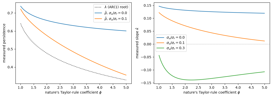
Fig. 109.8 What the Fed’s regression measures under different policy rules#
The measured persistence \(\hat\rho\) lies well above the AR(1) root \(\lambda\), and all three fall as policy grows more aggressive.
With demand shocks only, \(\hat\kappa\) also falls with \(\phi\) but stays above the structural slope \(\kappa = 0.1\), as the formula says.
Even modest cost-push shocks pull it down sharply, and below zero.
The model is a stylized quarterly one, so its numbers are not meant to match the Fed’s estimates from four-quarter inflation.
109.8.3. The self-confirming fixed point#
Now compose the two maps.
A history of policy \(\phi\) produces measured beliefs \((\hat\rho(\phi), \hat\kappa(\phi))\).
Fed into the Phelps problem, those beliefs recommend the inflation coefficient
A fixed point \(\phi^* = T(\phi^*)\) is a self-confirming equilibrium in the sense of Self-Confirming Equilibria.
At \(\phi^*\), the Fed’s rule solves its Phelps problem given its beliefs, and its beliefs satisfy the least-squares orthogonality conditions in the data that its rule generates.
We make two simplifications.
Nature’s rule uses only the inflation coefficient that the Phelps problem recommends.
We also hold the Fed’s IS beliefs at the illustrative values of the previous section, so the loop runs only through the Phillips curve.
Since \(\hat\rho\) and \(\hat\kappa\) fall as \(\phi\) rises, and \(\phi_\pi\) rises with both (for small \(\kappa\)), \(T\) is decreasing: the loop is a negative feedback.
def T(φ, **nature):
    "Inflation coefficient recommended by beliefs measured under the rule φ."
    _, ρ_hat, κ_hat = fed_regression(φ, **nature)
    return φ_π(ρ_hat, κ_hat)

def fixed_point(**nature):
    "φ* = T(φ*) and the slope T′(φ*)."
    φ_star = brentq(lambda φ: T(φ, **nature) - φ, 1.01, 5.0)
    h = 1e-5
    slope = (T(φ_star + h, **nature) - T(φ_star - h, **nature)) / (2 * h)
    return φ_star, slope

fig, ax = plt.subplots(figsize=(7, 4.5))
for σ_u in [0.0, 0.1]:
    ax.plot(φ_grid, [T(φ, σ_u=σ_u) for φ in φ_grid],
            label=rf'$T(\phi)$, $\sigma_u/\sigma_r = {σ_u}$')
ax.plot(φ_grid, φ_grid, 'k:', lw=1, label='45° line')
ax.set_xlabel(r'past policy $\phi$')
ax.set_ylabel(r'recommended $\phi_\pi$')
ax.legend()
plt.show()

cases = {'baseline': {}, 'σ_u/σ_r = 0.1': {'σ_u': 0.1},
         'ω = 0.5': {'ω': 0.5}, 'κ = 0.05': {'κ': 0.05}}
for name, nature in cases.items():
    φ_star, slope = fixed_point(**nature)
    _, ρ_hat, κ_hat = fed_regression(φ_star, **nature)
    print(f"{name:>15}: φ* = {φ_star:.3f}, T′(φ*) = {slope:.3f}, "
          f"beliefs (ρ̂, κ̂) = ({ρ_hat:.3f}, {κ_hat:.3f})")
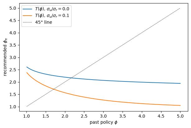
Fig. 109.9 The map from past policy to the policy the Phelps problem recommends#
       baseline: φ* = 2.166, T′(φ*) = -0.161, beliefs (ρ̂, κ̂) = (0.653, 0.130)
  σ_u/σ_r = 0.1: φ* = 1.708, T′(φ*) = -0.568, beliefs (ρ̂, κ̂) = (0.607, 0.082)
        ω = 0.5: φ* = 1.612, T′(φ*) = -0.076, beliefs (ρ̂, κ̂) = (0.434, 0.130)
       κ = 0.05: φ* = 1.871, T′(φ*) = -0.199, beliefs (ρ̂, κ̂) = (0.707, 0.070)
\(T\) crosses the 45-degree line once, so the self-confirming equilibrium is unique.
Is it stable under learning?
A Fed that learns with a small gain follows mean dynamics like \(d\phi/d\tau = T(\phi) - \phi\), the ordinary differential equation of One recursion, many learners.
The rest point is E-stable if \(T'(\phi^*) < 1\).
In belief space the same condition appears.
The map \((\rho, \kappa) \mapsto (\hat\rho, \hat\kappa)(\phi_\pi(\rho, \kappa))\) has a rank-one Jacobian whose nonzero eigenvalue is \(T'(\phi^*)\).
So the E-stability eigenvalues are \(-1\) and \(T'(\phi^*) - 1\), the kind of calculation that Self-Confirming Equilibria carries out for the Conquest’s model (Uniqueness and E-stability).
Because \(T' < 0\), the condition holds with room to spare in every case above.
Because \(|T'| < 1\) as well, even the gain-one “cobweb” iteration \(\phi_{k+1} = T(\phi_k)\) converges.
It describes a Fed that re-optimizes only after its beliefs have fully adjusted to each policy regime:
for name in ['baseline', 'σ_u/σ_r = 0.1']:
    φ_k, path = 3.0, [3.0]                     # start from an aggressive history
    for _ in range(8):
        φ_k = T(φ_k, **cases[name])
        path.append(φ_k)
    print(f"{name:>15}:", np.round(path, 2))
       baseline: [3.   2.07 2.18 2.16 2.17 2.17 2.17 2.17 2.17]
  σ_u/σ_r = 0.1: [3.   1.27 2.04 1.55 1.81 1.65 1.74 1.69 1.72]
An aggressive history is followed by a timid rule, then by a partial correction, in damped oscillations around \(\phi^*\).
That is a faint echo of “conquest lost and regained”, but it dies out.
109.8.4. A trap without an escape route#
The fixed point has the structure of the Conquest’s self-confirming equilibria.
The anticipated-utility Fed never experiments, by construction (Adaptive Learning and Escape Dynamics).
At \(\phi^*\) its beliefs are right on the equilibrium path and wrong off it: under a less aggressive rule, measured persistence and slope would rise.
This is the lack-of-experimentation trap of Escaping Nash Inflation (The experimentation trap), and it is the sense of the extended abstract’s framing.
The difference lies in the dynamics.
In the model of Cho et al. [2002], the escape route is self-reinforcing.
A run of shocks that steepens the perceived Phillips curve makes the government cut inflation, and that generates data that steepen the curve further.
Here the feedback runs the other way.
A run of shocks that raises measured persistence makes the Fed more aggressive, and more aggressive policy lowers measured persistence.
A constant-gain learner would wander around \(\phi^*\), but the mean dynamics pull it back from either side: there is no escape route.
Two facts also limit how much this loop can explain about the data.
First, in Fig. 109.1 the fall in \(\rho_t\) came after 2008, when the zero lower bound kept policy from being aggressive at all.
Second, the jump in \(\rho_t\) in 2022, alongside the inflation peak, is in line with the positive correlation between the level and the persistence of inflation that Drifts and Volatilities documents.
Escape-route models predict an inverse correlation; Cogley and Sargent [2005] (footnote 28) note that gradualism of the kind described above can produce the positive one.
So the 2020s were not a replay of the Conquest’s recurrent escapes.
What carries over is the Conquest’s diagnosis.
The Fed treated a reduced form whose coefficients depend on policy as if it were structural, ignoring the Lucas critique in just the way the vindication story of The Rise and Fall of U.S. Inflation describes (Sargent and Williams [2025], footnote 6).
But the misspecification now concerns the slope and persistence of the Phillips curve, not the natural-rate hypothesis.
Note
Sargent and Williams [2025] also acknowledge a very different reading in which the accommodation of the 2020s was fiscal in origin, as in the fiscal-theory accounts they cite.
That would be another rationalization of the same policy path.
109.9. Was the conquest lost?#
The Rise and Fall of U.S. Inflation ended by asking what the data since 1999 say about its two stories.
Would a credible low-inflation equilibrium keep re-anchoring after each shock, as the triumph of natural-rate theory suggests?
Or could surprises still set a monetary authority’s beliefs drifting, as the vindication of econometric policy evaluation suggests?
Following Sargent and Williams [2025], this lecture’s answer is that the conquest was lost for a while.
The reason was not a change in the Fed’s objectives.
The artificial Fed’s loss function never changes.
Its beliefs drifted during a long period of low and stable inflation, so that by 2019 its Phelps problem prescribed a long-run response to inflation only a little above one; that made its response to the surge muted.
Real-time measures of slack, which overstated how much room the economy had, made it late.
Once the 2022 data arrived, perceived persistence jumped back toward one, the rule’s response to inflation jumped with it, and the conquest was regained.
In the language of The Rise and Fall of U.S. Inflation, the episode looks like the vindication story’s adaptive policy maker, misled by a reduced form whose coefficients depend on policy.
But it is not a replay of that story’s recurrent escapes.
The policy-to-beliefs loop we built has no escape route; drifting beliefs explain why the response was muted, and mismeasured data explain why it was late.
Nor does anything here contradict the triumph story’s reading, recorded in The Rise and Fall of U.S. Inflation, that long-run inflation expectations stayed anchored: the artificial Fed’s beliefs concern the reduced-form dynamics of inflation, not the public’s expectations.
The lesson the episode adds to the Conquest is the one the extended abstract draws: the lessons of past successful policy can fade during long tranquil periods, and then have to be learned again.
109.10. Exercises#
Exercise 109.1
The interest-smoothing weight \(\eta\) in the loss (109.3) is, in the paper’s words, “one of the most important parameters.”
The paper says that a larger \(\eta\) fits the observed rate better but makes the rule harder to interpret as systematic stabilization policy.
Make that tradeoff quantitative.
For \(\eta \in \{0.1, 0.5, 2.0\}\):
compute the recommended rates and their root mean squared error (RMSE) against the actual funds rate from 1991 on, and compare with the no-change rule \(i_t = i_{t-1}\);
compute the 2019Q4 rule and its long-run response to inflation, \(\phi_\pi/(1 - \phi_i)\);
plot the recommendations against the actual rate from 2015 on.
Which \(\eta\) would you choose, and why?
Solution
The beliefs do not depend on \(\eta\), so we reuse them.
fig, ax = plt.subplots(figsize=(10, 4.5))
w = slice('2015', None)
print(f"{'η':>5} {'RMSE':>6} {'ϕ_π':>7} {'ϕ_i':>7} {'long run':>9}")
for η_val in [0.1, 0.5, 2.0]:
    rules_η = phelps_rules(beliefs, η=η_val)
    rate = recommended_rate(data, rules_η)
    f = rules_η.loc['2019-10-01']
    print(f"{η_val:>5} {fit(rate)[1]:>6.2f} {f.φ_π:>7.3f} {f.φ_i:>7.3f} "
          f"{f.φ_π / (1 - f.φ_i):>9.2f}")
    ax.plot(rate[w], lw=1, label=rf'$\eta = {η_val}$')
print(f"no-change rule RMSE: {fit(no_change)[1]:.2f}")
ax.plot(data['i'][w], 'k:', lw=1.5, label='actual')
ax.set_xlabel('year')
ax.set_ylabel('percent')
ax.legend()
plt.show()
    η   RMSE     ϕ_π     ϕ_i  long run
  0.1   1.76   0.297   0.862      2.15
  0.5   0.79   0.092   0.929      1.30
  2.0   0.47   0.030   0.966      0.88
no-change rule RMSE: 0.45
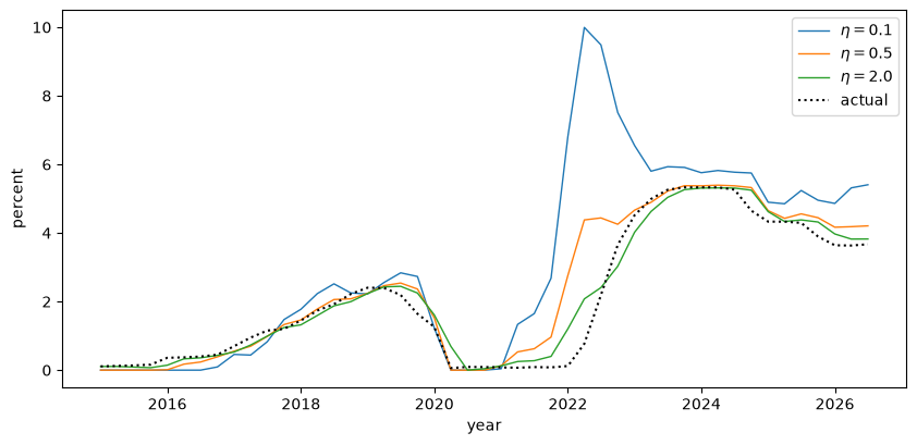
A small \(\eta\) produces a volatile rate that jumps sharply with inflation and the gap, and fits badly.
Raising \(\eta\) improves the fit a lot, but at \(\eta = 2\) the RMSE is close to that of the no-change rule.
Meanwhile the 2019 rule’s long-run response to inflation falls below one, so the rule no longer satisfies the Taylor principle.
A large \(\eta\) buys fit by turning the Phelps rule into a no-change rule.
That is the concrete meaning of the paper’s “interpretability.”
\(\eta = 0.5\) keeps a long-run response above one while fitting far better than \(\eta = 0.1\).
Exercise 109.2
This exercise explores the simplified Phelps problem (109.5).
Show that \(P_{12} = 0\) and \(P_{22} = \lambda_x\) solve its Riccati equation. (Hint: the second column of \(A\) is a multiple of \(B\).) Then derive the quadratic equation for \(P_{11}\), and confirm both results with
solve_discrete_are.For \(\rho \in \{0.5, 0.9\}\), plot \(\phi_\pi\) against \(\kappa \in (0, 3]\) and find the slope at which \(\phi_\pi\) peaks. Explain why \(\phi_\pi\) eventually falls as \(\kappa\) grows.
Add a penalty \(\eta_r r_t^2\) on the real rate to the loss. Does the reversal survive for \(\eta_r \in \{0.01, 0.1\}\)?
Solution
Part 1. With \(r_t\) as the control,
so the second column of \(A\) equals \((b_1/g) B\).
With no control cost, the Riccati equation is
The matrix in parentheses annihilates \(B\), so the second row and column of \(A^\top(\cdot)A\) vanish.
Hence \(P\) agrees with \(Q = \operatorname{diag}(1, \lambda_x)\) in its second row and column: \(P_{12} = 0\) and \(P_{22} = \lambda_x\).
Economically, the Fed can offset the predictable part of next quarter’s gap completely, so the current gap carries no cost into the future.
Using \(B^\top P B = g^2(\kappa^2 P_{11} + \lambda_x)\) and \((PB)_1 = g\kappa P_{11}\), the \((1,1)\) element gives
whose positive root is the paper’s equation (8); \(Z = \kappa^2 P_{11}\).
def riccati_P(ρ, κ, b1=0.9, g=-0.5, λ_x=0.2, β=0.95, η_r=1e-9):
    A = np.array([[ρ, κ * b1], [0, b1]])
    B = np.array([[κ * g], [g]])
    return solve_discrete_are(np.sqrt(β) * A, np.sqrt(β) * B,
                              np.diag([1, λ_x]), np.array([[η_r]]))

for ρ_, κ_ in [(0.9, 0.05), (0.5, 0.2), (0.95, 1.0)]:
    P = riccati_P(ρ_, κ_)
    Δ = 0.2 * (1 - 0.95 * ρ_**2) - κ_**2
    P11 = (-Δ + np.sqrt(Δ**2 + 4 * 0.2 * κ_**2)) / (2 * κ_**2)
    print(f"ρ = {ρ_}, κ = {κ_}: P12 = {P[0, 1]:.1e}, P22 = {P[1, 1]:.4f}, "
          f"P11 = {P[0, 0]:.4f} (closed form {P11:.4f})")
ρ = 0.9, κ = 0.05: P12 = 2.9e-09, P22 = 0.2000, P11 = 3.7715 (closed form 3.7715)
ρ = 0.5, κ = 0.2: P12 = 1.8e-09, P22 = 0.2000, P11 = 1.2353 (closed form 1.2353)
ρ = 0.95, κ = 1.0: P12 = 2.9e-09, P22 = 0.2000, P11 = 1.1460 (closed form 1.1460)
Parts 2 and 3.
κ_wide = np.linspace(0.005, 3.0, 600)
fig, ax = plt.subplots(figsize=(8, 4.5))
for ρ_ in [0.5, 0.9]:
    curve = φ_π(ρ_, κ_wide)
    ax.plot(κ_wide, curve, label=rf'$\rho = {ρ_}$, $\eta_r = 0$')
    print(f"ρ = {ρ_}, η_r = 0: peak at κ = {κ_wide[np.argmax(curve)]:.3f}")
for η_r in [0.01, 0.1]:
    curve = [φ_π_riccati(0.9, κ_, η_r=η_r) for κ_ in κ_wide]
    ax.plot(κ_wide, curve, '--', label=rf'$\rho = 0.9$, $\eta_r = {η_r}$')
    print(f"ρ = 0.9, η_r = {η_r}: peak at κ = {κ_wide[np.argmax(curve)]:.3f}, "
          f"monotone in κ: {np.all(np.diff(curve) > 0)}")
ax.set_xlabel(r'perceived slope $\kappa$')
ax.set_ylabel(r'$\phi_\pi$')
ax.legend()
plt.show()
ρ = 0.5, η_r = 0: peak at κ = 0.390
ρ = 0.9, η_r = 0: peak at κ = 0.215
ρ = 0.9, η_r = 0.01: peak at κ = 0.230, monotone in κ: False
ρ = 0.9, η_r = 0.1: peak at κ = 0.290, monotone in κ: False
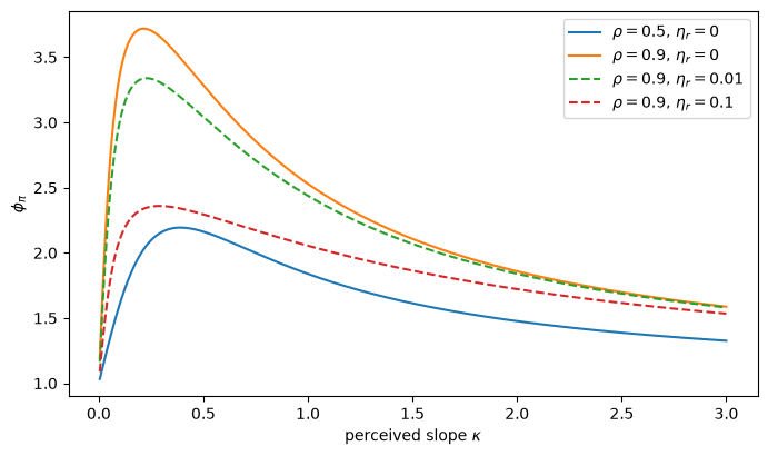
\(\phi_\pi\) is hump-shaped in \(\kappa\).
When the curve is very flat, moving inflation through the gap is expensive, so the Fed does little: \(Z/(Z + \lambda_x)\) is small.
When the curve is steep, a small change in the gap moves inflation a lot, so a small rate response suffices: \(\phi_\pi \approx 1 + \rho/(|g|\kappa)\) falls toward one.
The peak lies in between, at a smaller \(\kappa\) when \(\rho\) is larger.
The paper’s footnote 19 suggests that a small control cost makes \(\partial\phi_\pi/\partial\kappa > 0\) for all \(\kappa\).
Numerically the hump survives a penalty on the real rate, so Proposition 109.2 is best read as a statement about small slopes.
The slopes the Fed estimated in the 2010s lie inside that region.
Exercise 109.3
The baseline sets the gain to zero in both 2020 and 2021.
Recompute the beliefs and the recommended rates (a) freezing only 2020 and (b) with no freeze at all.
Report \(\rho_t\), \(\kappa_t\), and the recommended rate for 2021–2022.
Which part of the freeze drives the result, and what does setting the gain to zero in 2021 assume?
Solution
We loop over the three treatments of the pandemic quarters.
fig, ax = plt.subplots(figsize=(10, 4.5))
w = slice('2019', '2023')
for freeze, style in [((2020, 2021), '-'), ((2020,), '--'), ((), ':')]:
    b = estimate_beliefs(data, freeze=freeze)
    rate = recommended_rate(data, phelps_rules(b))
    label = f"freeze {freeze}" if freeze else 'no freeze'
    print(f"\n{label}")
    print(pd.DataFrame({'ρ': b['rho'], 'κ': b['kappa'], 'rate': rate})
            .loc['2021':'2022'].rename(index=qtr).round(3).T.to_string())
    ax.plot(rate[w], style, label=label)
ax.plot(data['i'][w], 'k', lw=1, alpha=0.6, label='actual')
ax.set_xlabel('year')
ax.set_ylabel('percent')
ax.legend()
plt.show()
freeze (2020, 2021)
      2021Q1  2021Q2  2021Q3  2021Q4  2022Q1  2022Q2  2022Q3  2022Q4
ρ      0.858   0.858   0.858   0.858   0.951   0.981   0.974   0.947
κ      0.039   0.039   0.039   0.039   0.048   0.047   0.047   0.048
rate   0.129   0.532   0.624   0.965   2.761   4.379   4.438   4.253

freeze (2020,)
      2021Q1  2021Q2  2021Q3  2021Q4  2022Q1  2022Q2  2022Q3  2022Q4
ρ      0.848   0.850   0.885   0.944   0.989   0.995   0.974   0.940
κ      0.042   0.076   0.084   0.106   0.107   0.106   0.109   0.113
rate   0.184   1.097   1.839   5.026   8.048   8.502   7.400   6.400

no freeze
      2021Q1  2021Q2  2021Q3  2021Q4  2022Q1  2022Q2  2022Q3  2022Q4
ρ      0.823   0.831   0.869   0.933   0.980   0.985   0.965   0.931
κ      0.078   0.102   0.107   0.121   0.121   0.120   0.122   0.125
rate   0.283   1.268   2.028   5.090   7.875   8.251   7.297   6.438
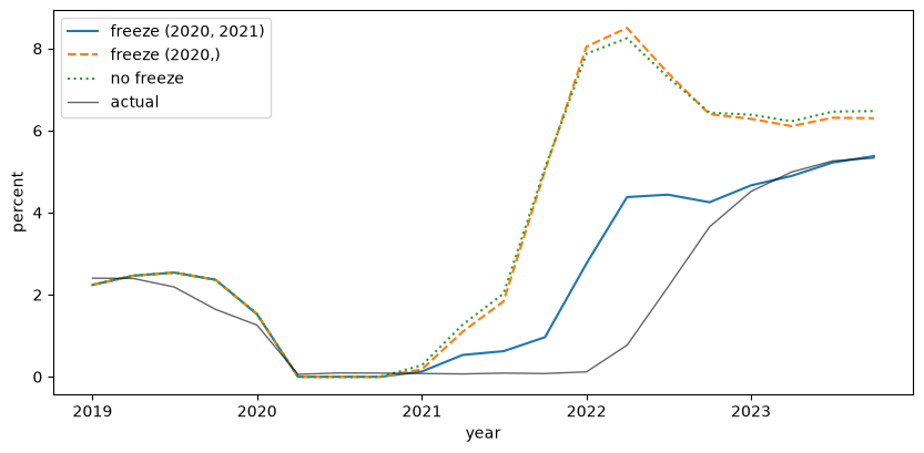
Freezing only 2020 gives almost the same answer as no freeze at all: the extreme 2020 quarters are not what matter.
What matters is 2021.
A Fed that learned from 2021 would have seen inflation rise with a positive gap, so its perceived slope \(\kappa_t\) would have steepened sharply and its perceived persistence would have risen.
Its recommended rate would have reached several percent by the end of 2021.
So the baseline’s zero gain in 2021 builds in the judgment that the 2021 data were uninformative about inflation dynamics, which is the “transitory” view itself.
The freeze is a modeling choice that helps the model rationalize a slow Fed, not a neutral treatment of outliers.
Exercise 109.4
Chung [1990] treated the gain of a government’s learning algorithm as a free parameter to be estimated (Exercise 91.7).
Econometric Policy Evaluation takes up his problem on 1960–1995 data.
Pose Chung’s problem for the artificial Fed.
For gains \(\gamma\) between \(0.01\) and \(0.05\), recompute the beliefs and recommendations and the RMSE against the actual rate from 1991 on.
Which gain fits best?
What happens to beliefs and recommendations in 2022 at \(\gamma = 0.05\)?
Solution
We keep track of the largest perceived persistence and the largest recommendation in 2022–2023 for each gain.
gains = np.arange(0.01, 0.0501, 0.005)
rmse, extremes = [], {}
for γ_val in gains:
    b = estimate_beliefs(data, γ=γ_val)
    rate = recommended_rate(data, phelps_rules(b))
    rmse.append(fit(rate)[1])
    extremes[round(γ_val, 3)] = (b['rho']['2022':'2023'].max(),
                                 rate['2022':'2023'].max())

fig, ax = plt.subplots(figsize=(7, 4))
ax.plot(gains, rmse, marker='o')
ax.set_xlabel(r'gain $\gamma$')
ax.set_ylabel('RMSE, 1991 on')
plt.show()

print(f"best gain on the grid: {gains[np.argmin(rmse)]:.3f}")
for γ_val in [0.03, 0.05]:
    ρ_max, rate_max = extremes[γ_val]
    print(f"γ = {γ_val}: max ρ_t in 2022-23 = {ρ_max:.3f}, "
          f"max recommended rate = {rate_max:.1f}%")
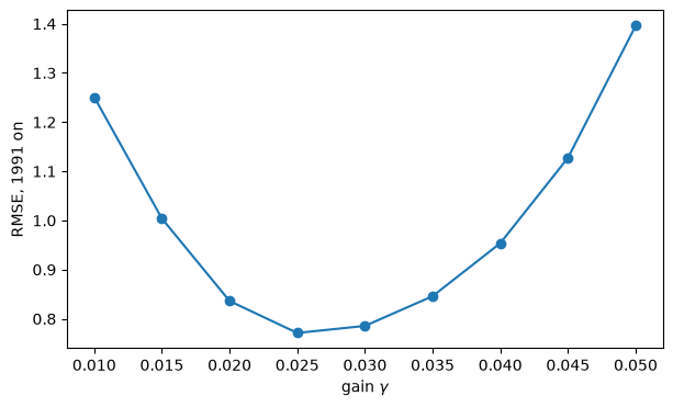
best gain on the grid: 0.025
γ = 0.03: max ρ_t in 2022-23 = 0.981, max recommended rate = 5.4%
γ = 0.05: max ρ_t in 2022-23 = 1.036, max recommended rate = 11.9%
The best fit is close to the paper’s \(\gamma = 0.03\).
Small gains make beliefs too sluggish to follow the drift.
Large gains make them chase noise.
At \(\gamma = 0.05\), the 2022 surprises push perceived persistence above one: the Fed’s model becomes explosive, and its Phelps problem calls for an enormous tightening.
The larger the gain, the more a few quarters of surprises can transform the Fed’s model.
This criterion is a least-squares fit of the policy rate that treats the loss parameters as known, not Chung’s likelihood for the whole system.
Exercise 109.5
This exercise reconciles the persistence measure of this lecture with the one in Drifts and Volatilities (Inflation persistence).
Show by simulation that if quarterly inflation were serially uncorrelated, a regression of four-quarter inflation on its one-quarter lag would give a coefficient near \(0.75\).
Rerun
estimate_beliefswith quarterly annualized inflation \(400 \log(P_t/P_{t-1})\) in place of four-quarter inflation, and compare the two paths of \(\rho_t\).When does persistence fall under each measure?
Solution
We start with the overlap, then rerun the beliefs on quarterly data.
rng = np.random.default_rng(0)
quarterly = rng.standard_normal(100_000)
four_quarter = np.convolve(quarterly, np.ones(4) / 4, mode='valid')
coef = np.polyfit(four_quarter[:-1], four_quarter[1:], 1)[0]
print(f"regression coefficient with IID quarterly inflation: {coef:.3f}")

data_q = data.copy()
data_q['pi'] = 400 * np.log(pce / pce.shift(1))[data.index]
beliefs_q = estimate_beliefs(data_q)

fig, ax = plt.subplots(figsize=(10, 4.5))
ax.plot(beliefs['rho'], label='four-quarter inflation (baseline)')
ax.plot(beliefs_q['rho'], label='quarterly annualized inflation')
ax.axhline(0.75, color='k', lw=0.5, ls=':')
ax.set_xlabel('year')
ax.set_ylabel(r'perceived persistence $\rho_t$')
ax.legend()
plt.show()

dates = ['1980-01-01', '1985-01-01', '1995-01-01', '2005-01-01',
         '2015-01-01', '2019-10-01', '2022-04-01']
print(pd.DataFrame({'four-quarter': beliefs['rho'], 'quarterly': beliefs_q['rho']})
        .loc[dates].rename(index=qtr).round(2).T.to_string())
regression coefficient with IID quarterly inflation: 0.749
              1980Q1  1985Q1  1995Q1  2005Q1  2015Q1  2019Q4  2022Q2
four-quarter    1.02    0.98    0.98    0.96    0.85    0.86    0.98
quarterly       0.94    0.86    0.83    0.74    0.46    0.39    0.64
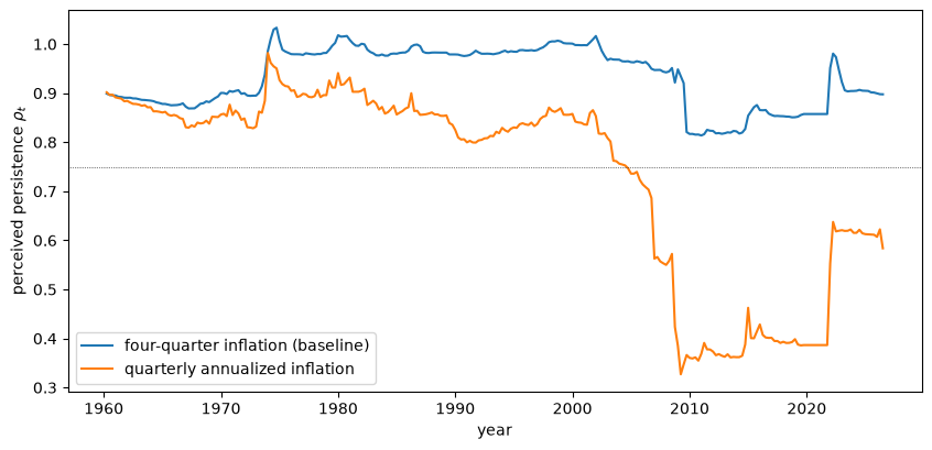
The overlap of four-quarter rates builds in a coefficient of about \(0.75\) even without any persistence in quarterly inflation, so the baseline \(\rho_t\) cannot fall far.
With quarterly inflation, persistence falls modestly after 1980, further by the mid-2000s, and to around 0.4 in the 2010s.
It rises again in 2022, but to a level far below one.
The overlap thus both inflates the level of the baseline measure and hides the early part of its decline.
The quarterly measure is closer to Drifts and Volatilities, which finds persistence falling soon after 1980.
Both measures agree on the main fact this lecture uses: by 2019 inflation was much less persistent than it had been.