24. Likelihood Processes For VAR Models#
24.1. Overview#
This lecture extends our analysis of likelihood ratio processes to Vector Autoregressions (VARs).
We’ll
Construct likelihood functions for VAR models
Form likelihood ratio processes for comparing two VAR models
Visualize the evolution of likelihood ratios over time
Compute the Kullback–Leibler divergence rate that governs the drift of a log likelihood ratio
Connect VAR likelihood ratios to the Samuelson multiplier-accelerator model
Our analysis builds on concepts from:
Let’s start by importing helpful libraries:
import numpy as np
import matplotlib.pyplot as plt
from scipy import linalg
from scipy.stats import multivariate_normal as mvn
from collections import namedtuple

rng = np.random.default_rng(1234)
24.2. VAR model setup#
Consider a VAR model of the form:
where:
\(x_t\) is an \(n \times 1\) state vector
\(w_{t+1} \sim \mathcal{N}(0, I)\) is an \(m \times 1\) vector of shocks
\(A\) is an \(n \times n\) transition matrix
\(C\) is an \(n \times m\) volatility matrix
Let’s define the necessary data structures for the VAR model
VARModel = namedtuple('VARModel', ['A', 'C', 'μ_0', 'Σ_0',
                                    'CC', 'CC_inv', 'log_det_CC',
                                    'Σ_0_inv', 'log_det_Σ_0'])
def compute_stationary_var(A, C):
    """
    Compute stationary mean and covariance for VAR model
    """
    n = A.shape[0]

    # Check stability
    eigenvalues = np.linalg.eigvals(A)
    if np.max(np.abs(eigenvalues)) >= 1:
        raise ValueError("VAR is not stationary")

    μ_0 = np.zeros(n)

    # Stationary covariance: solve discrete Lyapunov equation
    # Σ_0 = A @ Σ_0 @ A.T + C @ C.T
    CC = C @ C.T
    Σ_0 = linalg.solve_discrete_lyapunov(A, CC)

    return μ_0, Σ_0

def create_var_model(A, C, μ_0=None, Σ_0=None, stationary=True):
    """
    Create a VAR model with parameters and precomputed matrices
    """
    A = np.asarray(A)
    C = np.asarray(C)
    n = A.shape[0]
    CC = C @ C.T

    if stationary:
        μ_0_comp, Σ_0_comp = compute_stationary_var(A, C)
    else:
        μ_0_comp = μ_0 if μ_0 is not None else np.zeros(n)
        Σ_0_comp = Σ_0 if Σ_0 is not None else np.eye(n)

    # Check if CC is singular
    det_CC = np.linalg.det(CC)
    if np.abs(det_CC) < 1e-10:
        # Use pseudo-inverse for singular case
        CC_inv = np.linalg.pinv(CC)
        CC_reg = CC + 1e-10 * np.eye(CC.shape[0])
        log_det_CC = np.log(np.linalg.det(CC_reg))
    else:
        CC_inv = np.linalg.inv(CC)
        log_det_CC = np.log(det_CC)

    # Same check for Σ_0
    det_Σ_0 = np.linalg.det(Σ_0_comp)
    if np.abs(det_Σ_0) < 1e-10:
        Σ_0_inv = np.linalg.pinv(Σ_0_comp)
        Σ_0_reg = Σ_0_comp + 1e-10 * np.eye(Σ_0_comp.shape[0])
        log_det_Σ_0 = np.log(np.linalg.det(Σ_0_reg))
    else:
        Σ_0_inv = np.linalg.inv(Σ_0_comp)
        log_det_Σ_0 = np.log(det_Σ_0)

    return VARModel(A=A, C=C, μ_0=μ_0_comp, Σ_0=Σ_0_comp,
                    CC=CC, CC_inv=CC_inv, log_det_CC=log_det_CC,
                    Σ_0_inv=Σ_0_inv, log_det_Σ_0=log_det_Σ_0)
24.2.1. Joint distribution#
The joint probability density \(p(x_T, x_{T-1}, \ldots, x_0)\) can be factored as:
Since the VAR is Markovian, \(p(x_{t+1} | x_t, \ldots, x_0) = p(x_{t+1} | x_t)\).
We write \(p\) for a generic density and reserve \(f\) and \(g\) for the names of two models.
24.2.2. Conditional densities#
Given the Gaussian structure, the conditional distribution \(p(x_{t+1} | x_t)\) is Gaussian with:
Mean: \(A x_t\)
Covariance: \(CC^\top\)
The log conditional density is
def log_likelihood_transition(x_next, x_curr, model):
    """
    Compute log likelihood of transition from x_curr to x_next
    """
    x_next = np.atleast_1d(x_next)
    x_curr = np.atleast_1d(x_curr)
    n = len(x_next)
    diff = x_next - model.A @ x_curr
    return -0.5 * (n * np.log(2 * np.pi) + model.log_det_CC +
                  diff @ model.CC_inv @ diff)
The log density of the initial state is:
def log_likelihood_initial(x_0, model):
    """
    Compute log likelihood of initial state
    """
    x_0 = np.atleast_1d(x_0)
    n = len(x_0)
    diff = x_0 - model.μ_0
    return -0.5 * (n * np.log(2 * np.pi) + model.log_det_Σ_0 +
                  diff @ model.Σ_0_inv @ diff)
The following function simulates paths from a VAR model
def simulate_var(model, T, rng, N_paths=1):
    """
    Simulate paths from the VAR model
    """
    n = model.A.shape[0]
    m = model.C.shape[1]
    paths = np.zeros((N_paths, T+1, n))

    for i in range(N_paths):
        # Draw initial state
        x = mvn.rvs(mean=model.μ_0, cov=model.Σ_0, random_state=rng)
        x = np.atleast_1d(x)
        paths[i, 0] = x

        # Simulate forward
        for t in range(T):
            w = rng.standard_normal(m)
            x = model.A @ x + model.C @ w
            paths[i, t+1] = x

    return paths if N_paths > 1 else paths[0]
24.3. Likelihood ratio process#
Now let’s compute likelihood ratio processes for comparing two VAR models \(f\) and \(g\).
Let \(p_f\) and \(p_g\) denote densities under models \(f\) and \(g\) respectively.
As in Likelihood Ratio Processes, \(L_t\) denotes the likelihood ratio of the sample \(x_0, x_1, \ldots, x_t\):
where the conditional densities are given by (24.1) and the densities of \(x_0\) by (24.2).
The log likelihood ratio process is
It obeys the recursion \(\log L_t = \log L_{t-1} + \ell_t\) with initial condition \(\log L_0 = \log p_f(x_0) - \log p_g(x_0)\).
Let’s write those equations in Python
def compute_likelihood_ratio_var(paths, model_f, model_g):
    """
    Compute likelihood ratio process for VAR models
    """
    if paths.ndim == 2:
        paths = paths[np.newaxis, :]

    N_paths, T_plus_1, n = paths.shape
    T = T_plus_1 - 1
    log_L_ratios = np.zeros((N_paths, T+1))

    for i in range(N_paths):
        X = paths[i]

        # Initial log likelihood ratio
        log_L_f_0 = log_likelihood_initial(X[0], model_f)
        log_L_g_0 = log_likelihood_initial(X[0], model_g)
        log_L_ratios[i, 0] = log_L_f_0 - log_L_g_0

        # Recursive computation
        for t in range(1, T+1):
            log_L_f_t = log_likelihood_transition(X[t], X[t-1], model_f)
            log_L_g_t = log_likelihood_transition(X[t], X[t-1], model_g)

            # Update log likelihood ratio
            log_diff = log_L_f_t - log_L_g_t

            log_L_prev = log_L_ratios[i, t-1]
            log_L_new = log_L_prev + log_diff
            log_L_ratios[i, t] = log_L_new

    return log_L_ratios if N_paths > 1 else log_L_ratios[0]
24.4. Example 1: two AR(1) processes#
Let’s start with a simple example comparing two univariate AR(1) processes with \(A_f = 0.8\), \(A_g = 0.5\), and \(C_f = 0.3\), \(C_g = 0.4\)
# Model f: AR(1) with persistence ρ = 0.8
A_f = np.array([[0.8]])
C_f = np.array([[0.3]])

# Model g: AR(1) with persistence ρ = 0.5
A_g = np.array([[0.5]])
C_g = np.array([[0.4]])

# Create VAR models
model_f = create_var_model(A_f, C_f)
model_g = create_var_model(A_g, C_g)
Let’s generate 100 paths of length 200 from model \(f\) and compute the likelihood ratio processes
# Simulate from model f
T = 200
N_paths = 100
paths_from_f = simulate_var(model_f, T, rng, N_paths)

L_ratios_f = compute_likelihood_ratio_var(paths_from_f, model_f, model_g)

fig, ax = plt.subplots()

for i in range(min(20, N_paths)):
    ax.plot(L_ratios_f[i], alpha=0.3, color='C0', lw=2)

ax.axhline(y=0, color='gray', linestyle='--', alpha=0.5)
ax.set_ylabel(r'$\log L_t$')
ax.set_title('log likelihood ratio processes (nature = f)')

plt.tight_layout()
plt.show()
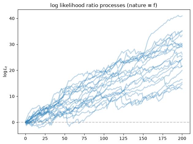
As we expected, the log likelihood ratio processes go to \(+\infty\) as \(t\) increases, indicating that model \(f\) is chosen correctly by our algorithm.
24.5. Example 2: bivariate VAR models#
Now let’s consider an example with bivariate VAR models with
and
A_f = np.array([[0.7, 0.2],
                 [0.1, 0.6]])

C_f = np.array([[0.3, 0.1],
                 [0.1, 0.3]])

A_g = np.array([[0.5, 0.3],
                 [0.2, 0.5]])

C_g = np.array([[0.4, 0.0],
                 [0.0, 0.4]])

# Create VAR models
model2_f = create_var_model(A_f, C_f)
model2_g = create_var_model(A_g, C_g)

# Check stationarity
print("model f eigenvalues:", np.linalg.eigvals(A_f))
print("model g eigenvalues:", np.linalg.eigvals(A_g))
model f eigenvalues: [0.8 0.5]
model g eigenvalues: [0.74494897 0.25505103]
Let’s generate 50 paths of length 50 from both models and compute the likelihood ratio processes
# Simulate from both models
T = 50
N_paths = 50

paths_from_f = simulate_var(model2_f, T, rng, N_paths)
paths_from_g = simulate_var(model2_g, T, rng, N_paths)

# Compute likelihood ratios
L_ratios_ff = compute_likelihood_ratio_var(paths_from_f, model2_f, model2_g)
L_ratios_gf = compute_likelihood_ratio_var(paths_from_g, model2_f, model2_g)
# Visualize the results
fig, axes = plt.subplots(1, 2, figsize=(12, 5))

ax = axes[0]
for i in range(min(20, N_paths)):
    ax.plot(L_ratios_ff[i], alpha=0.5, color='C0', lw=2)
ax.axhline(y=0, color='gray', linestyle='--', alpha=0.5, lw=2)
ax.set_title(r'$\log L_t$ (nature = f)')
ax.set_ylabel(r'$\log L_t$')

ax = axes[1]
for i in range(min(20, N_paths)):
    ax.plot(L_ratios_gf[i], alpha=0.5, color='C1', lw=2)
ax.axhline(y=0, color='gray', linestyle='--', alpha=0.5, lw=2)
ax.set_title(r'$\log L_t$ (nature = g)')
plt.tight_layout()
plt.show()
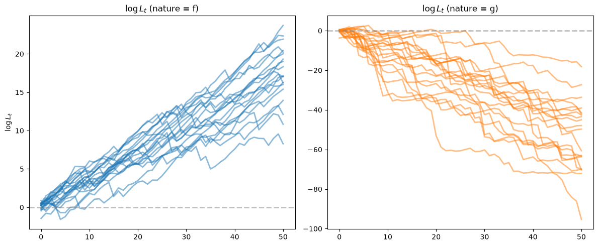
For paths generated from model \(f\), the log likelihood ratio processes tend to go to \(+\infty\), while for paths from model \(g\), they tend to go to \(-\infty\).
The paths fall faster under \(g\) than they rise under \(f\); the section KL divergence rate explains why.
Let’s apply the decision rule described in the section on model selection mistake probability in Likelihood Ratio Processes: select model \(f\) when \(\log L_T \geq 0\) and model \(g\) when \(\log L_T < 0\).
This rule is a likelihood ratio test with threshold \(L_T = 1\).
Suppose that a Bayesian puts prior probability \(1/2\) on each model.
Then the posterior probability of model \(f\) is \(L_T/(1 + L_T)\), as in Likelihood Ratio Processes and Bayesian Learning.
The rule selects the model with the higher posterior probability, so it minimizes the probability \(\frac{1}{2}(\alpha_T + \beta_T)\) of selecting the wrong model, where \(\alpha_T = {\rm Prob}(\log L_T < 0 | f)\) and \(\beta_T = {\rm Prob}(\log L_T \geq 0 | g)\).
fig, ax = plt.subplots()
T_values = np.arange(0, T+1)
accuracy_f = np.zeros(len(T_values))
accuracy_g = np.zeros(len(T_values))

for i, t in enumerate(T_values):
    # Correct selection when data from f
    accuracy_f[i] = np.mean(L_ratios_ff[:, t] > 0)
    # Correct selection when data from g
    accuracy_g[i] = np.mean(L_ratios_gf[:, t] < 0)

ax.plot(T_values, accuracy_f, 'C0', linewidth=2, label='accuracy (nature = f)')
ax.plot(T_values, accuracy_g, 'C1', linewidth=2, label='accuracy (nature = g)')
ax.axhline(y=0.5, color='gray', linestyle='--', alpha=0.5)
ax.set_xlabel('T')
ax.set_ylabel('accuracy')
ax.legend()

plt.tight_layout()
plt.show()
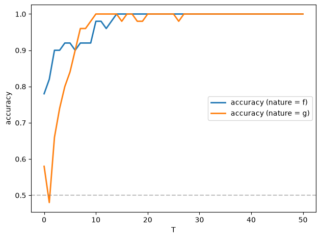
Evidently, the accuracy approaches \(1\) as \(T\) increases, and it does so very quickly.
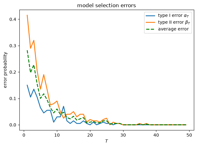
Let’s also check the type I and type II errors \(\alpha_T\) and \(\beta_T\) as functions of \(T\)
def model_selection_analysis(T_values, model_f, model_g, N_sim=500):
    """
    Analyze model selection performance for different sample sizes
    """
    errors_f = []  # Type I errors
    errors_g = []  # Type II errors

    for T in T_values:
        # Simulate from model f
        paths_f = simulate_var(model_f, T, rng, N_sim//2)
        L_ratios_f = compute_likelihood_ratio_var(paths_f, model_f, model_g)

        # Simulate from model g
        paths_g = simulate_var(model_g, T, rng, N_sim//2)
        L_ratios_g = compute_likelihood_ratio_var(paths_g, model_f, model_g)

        # Decision rule: choose f if log L_T >= 0
        errors_f.append(np.mean(L_ratios_f[:, -1] < 0))
        errors_g.append(np.mean(L_ratios_g[:, -1] >= 0))

    return np.array(errors_f), np.array(errors_g)

T_values = np.arange(1, 50, 1)
errors_f, errors_g = model_selection_analysis(T_values, model2_f, model2_g, N_sim=400)

fig, ax = plt.subplots()

ax.plot(T_values, errors_f, 'C0', linewidth=2, label=r'type I error $\alpha_T$')
ax.plot(T_values, errors_g, 'C1', linewidth=2, label=r'type II error $\beta_T$')
ax.plot(T_values, 0.5 * (errors_f + errors_g), 'g--',
linewidth=2, label='average error')
ax.set_xlabel('$T$')
ax.set_ylabel('error probability')
ax.set_title('model selection errors')
ax.legend()
plt.tight_layout()
plt.show()
The decision rule above fixes the sample size \(T\) in advance.
Wald’s sequential probability ratio test, described in A Problem that Stumped Milton Friedman, instead stops sampling the first time \(\log L_t\) leaves an interval.
Exercise Exercise 26.2 of that lecture applies it to two VAR models.
24.6. KL divergence rate#
The average slopes of the log likelihood ratio paths in the figures above are Kullback–Leibler divergence rates.
They are VAR counterparts of the KL divergence rate for Markov chains in Likelihood Ratio Processes.
Statistical Divergence Measures describes Kullback–Leibler divergence.
Let \(\Sigma_f = C_f C_f^\top\) and \(\Sigma_g = C_g C_g^\top\), and let \(V_f\) solve the discrete Lyapunov equation
so that \(\mathcal{N}(0, V_f)\) is the stationary distribution of \(x_t\) under model \(f\).
Suppose that model \(f\) generates the data and that \(x_0\) is drawn from \(\mathcal{N}(0, V_f)\), as in Examples 1 and 2.
Then every increment \(\ell_t\) in (24.3) has the same expected value
The first three terms in the brackets measure the discrepancy between the shock covariance matrices \(\Sigma_f\) and \(\Sigma_g\).
The last term measures the discrepancy between the conditional means \(A_f x_{t-1}\) and \(A_g x_{t-1}\), averaged over the stationary distribution of \(x_{t-1}\).
Because \(\{x_t\}\) is ergodic under \(f\),
When model \(g\) generates the data, \(\frac{1}{t} \log L_t \to -h_{KL}(g, f)\), where \(h_{KL}(g, f)\) is (24.4) with the roles of \(f\) and \(g\) reversed.
Exercise Exercise 24.1 asks you to derive (24.4) and to verify these limits by simulation.
The function below computes the two parts of (24.4).
It takes \(V_f\) from model_f.Σ_0, so model_f must be created with stationary=True.
def kl_rate_terms(model_f, model_g):
    """
    Covariance and conditional-mean terms of the KL divergence rate
    h_KL(f, g), with x_t drawn from the stationary distribution of model f
    """
    n = model_f.A.shape[0]
    D = model_f.A - model_g.A
    V_f = model_f.Σ_0
    cov_term = 0.5 * (np.trace(model_g.CC_inv @ model_f.CC) - n
                      + model_g.log_det_CC - model_f.log_det_CC)
    mean_term = 0.5 * np.trace(model_g.CC_inv @ D @ V_f @ D.T)
    return cov_term, mean_term

def kl_rate_var(model_f, model_g):
    """
    KL divergence rate h_KL(f, g) between two stationary Gaussian VARs
    """
    return sum(kl_rate_terms(model_f, model_g))

examples = [("Example 1", model_f, model_g),
            ("Example 2", model2_f, model2_g)]

for name, m_f, m_g in examples:
    for label, m1, m2 in [("h_KL(f, g)", m_f, m_g), ("h_KL(g, f)", m_g, m_f)]:
        cov_term, mean_term = kl_rate_terms(m1, m2)
        print(f"{name}: {label} = {cov_term + mean_term:.4f}  "
              f"(covariance terms {cov_term:.4f}, mean term {mean_term:.4f})")
Example 1: h_KL(f, g) = 0.1392  (covariance terms 0.0689, mean term 0.0703)
Example 1: h_KL(g, f) = 0.2079  (covariance terms 0.1012, mean term 0.1067)
Example 2: h_KL(f, g) = 0.3443  (covariance terms 0.3181, mean term 0.0261)
Example 2: h_KL(g, f) = 0.9614  (covariance terms 0.8069, mean term 0.1546)
For Example 2, \(h_{KL}(g, f) = 0.961\) is almost three times \(h_{KL}(f, g) = 0.344\).
That is why \(\log L_t\) falls faster when \(g\) generates the data than it rises when \(f\) generates the data.
The covariance terms account for most of both rates.
Both models assign variance \(0.16\) to the shock to \((x_{1t} + x_{2t})/\sqrt{2}\).
Model \(g\) assigns variance \(0.16\) to the shock to \((x_{1t} - x_{2t})/\sqrt{2}\); model \(f\) assigns it variance \(0.04\).
Let \(r\) be the variance of the shock to \((x_{1t} - x_{2t})/\sqrt{2}\) under the model that generates the data divided by its variance under the other model.
Because the two models agree about the other direction, the covariance terms equal \(\frac{1}{2}(r - 1 - \log r)\).
This expression equals \(0.807\) for \(r = 4\) (nature \(= g\)) and \(0.318\) for \(r = 1/4\) (nature \(= f\)).
Kullback–Leibler divergence penalizes a model that understates a variance more heavily than a model that overstates it.
In Example 1, the two parts contribute about equally, and \(h_{KL}(g, f) = 0.208\) exceeds \(h_{KL}(f, g) = 0.139\).
Let’s compare the theoretical rates for Example 2 with sample averages of \(\frac{1}{T} \log L_T\) across the paths simulated above
T2 = L_ratios_ff.shape[1] - 1

print(f"nature = f: mean of log L_T / T = {L_ratios_ff[:, -1].mean() / T2:.4f}, "
      f"h_KL(f, g) = {kl_rate_var(model2_f, model2_g):.4f}")
print(f"nature = g: mean of log L_T / T = {L_ratios_gf[:, -1].mean() / T2:.4f}, "
      f"-h_KL(g, f) = {-kl_rate_var(model2_g, model2_f):.4f}")
nature = f: mean of log L_T / T = 0.3472, h_KL(f, g) = 0.3443
nature = g: mean of log L_T / T = -0.9924, -h_KL(g, f) = -0.9614
The sample averages include the initial-condition term \(\log L_0\) divided by \(T = 50\), so they need not equal the rates exactly.
The KL rates describe the means of the increments \(\ell_t\).
Error probabilities for small \(T\) depend on the entire distribution of \(\log L_T\).
for nature, L_ratios in [('f', L_ratios_ff), ('g', L_ratios_gf)]:
    ℓ = np.diff(L_ratios, axis=1).ravel()
    print(f"nature = {nature}: increments ℓ_t have mean {ℓ.mean():.2f}, "
          f"median {np.median(ℓ):.2f}, standard deviation {ℓ.std():.2f}")
nature = f: increments ℓ_t have mean 0.34, median 0.53, standard deviation 0.54
nature = g: increments ℓ_t have mean -0.98, median -0.07, standard deviation 2.35
Under \(g\), the increments \(\ell_t\) have a mean near \(-1\), a median near \(0\), and a large standard deviation.
Under \(f\), their median exceeds their mean and their standard deviation is small.
That is why \(\beta_T\) exceeds \(\alpha_T\) for small \(T\) in the error-probability figure above, although \(\log L_t\) falls faster under \(g\) than it rises under \(f\).
24.7. Application: Samuelson multiplier-accelerator#
Now let’s connect to the Samuelson multiplier-accelerator model.
The model consists of:
Consumption: \(C_t = \gamma + a Y_{t-1}\) where \(a \in (0,1)\) is the marginal propensity to consume
Investment: \(I_t = b(Y_{t-1} - Y_{t-2}) + \sigma \epsilon_t\) where \(b > 0\) is the accelerator coefficient and \(\{\epsilon_t\}\) is an IID sequence of standard normal random variables
Government spending: \(G_t = G\) (constant)
We have the national income identity
Samuelson Multiplier-Accelerator writes \(\alpha\) and \(\beta\) for \(a\) and \(b\).
That lecture adds the shock \(\sigma \epsilon_t\) directly to the second-order difference equation for \(Y_t\).
We put the shock in the investment equation.
This leads to the same difference equation for \(Y_t\) and also determines how \(C_t\) and \(I_t\) respond to \(\epsilon_t\).
Substituting the consumption and investment equations into the national income identity yields the second-order difference equation:
With \(\rho_1 = a + b\) and \(\rho_2 = -b\), we have:
When the roots of \(z^2 - \rho_1 z - \rho_2\) lie inside the unit circle, \(Y_t\) has a stationary distribution with mean
When \(\sigma = 0\), \(Y_t\) converges to the steady state \(Y^*\), where investment is zero and \(Y^* = \gamma + a Y^* + G\).
To fit into our discussion, we write it into state-space representation.
To handle the constant term properly, we use an augmented state vector \(x_t = [1, Y_t, Y_{t-1}]^\top\):
The observation equation extracts the economic variables:
This gives us:
\(Y_t\) (total output)
\(C_t = \gamma \cdot 1 + a Y_{t-1}\) (consumption)
\(I_t = Y_t - C_t - G = b(Y_{t-1} - Y_{t-2}) + \sigma \epsilon_t\) (investment)
The third row uses the national income identity to recover \(I_t\) from \(Y_t\) and \(Y_{t-1}\), so the state vector need not include \(Y_{t-2}\).
The matrix \(CC^\top\) has rank one: given \(x_t\), the first and third components of \(x_{t+1}\) are known and only \(Y_{t+1}\) is random.
Consequently (24.1) is not a density with respect to Lebesgue measure on \(\mathbb{R}^3\).
create_var_model replaces \((CC^\top)^{-1}\) with a pseudo-inverse and adds \(10^{-10} I\) to \(CC^\top\) before taking the log determinant.
The regularization terms cancel in \(\ell_{t+1}\), which equals the log ratio of the conditional densities of \(Y_{t+1}\) given \(x_t\) under the two models.
The same device handles the singular covariance matrix \(\Sigma_0\) of \(x_0\), whose first component is always \(1\).
An econometrician who observes \(Y_t\) and \(Y_{t-1}\) observes the state \(x_t\).
When an econometrician observes only some components of a state vector, or observes them with error, a Kalman filter produces innovations from which to compute the likelihood, as in A First Look at the Kalman Filter and The Kalman Filter and Vector Autoregressions.
def samuelson_to_var(a, b, γ, G, σ):
    """
    Convert Samuelson model parameters to VAR form with augmented state

    Samuelson model:
    - Y_t = C_t + I_t + G
    - C_t = γ + a*Y_{t-1}
    - I_t = b*(Y_{t-1} - Y_{t-2}) + σ*ε_t

    Reduced form: Y_t = (γ+G) + (a+b)*Y_{t-1} - b*Y_{t-2} + σ*ε_t

    State vector is [1, Y_t, Y_{t-1}]'
    """
    ρ_1 = a + b
    ρ_2 = -b

    # State transition matrix for augmented state
    A = np.array([[1,      0,     0],
                  [γ + G,  ρ_1,   ρ_2],
                  [0,      1,     0]])

    # Shock loading matrix
    C = np.array([[0],
                  [σ],
                  [0]])

    # Observation matrix (extracts Y_t, C_t, I_t from [1, Y_t, Y_{t-1}]')
    G_obs = np.array([[0,         1,   0],    # Y_t
                      [γ,         0,   a],    # C_t = γ + a Y_{t-1}
                      [-(γ + G),  1,  -a]])   # I_t = Y_t - C_t - G

    return A, C, G_obs
We define functions in the code cell below to get the initial conditions and check stability
With stationary_init=True, the initial state \([1, Y_0, Y_{-1}]^\top\) has the stationary distribution: \((Y_0, Y_{-1})\) has mean \((Y^*, Y^*)\) and a covariance matrix that solves a discrete Lyapunov equation.
Let’s implement it and inspect the likelihood ratio processes induced by two Samuelson models with different parameters.
def create_samuelson_var_model(a, b, γ, G, σ, stationary_init=False,
                               y_0=None, y_m1=None):
    """
    Create a VAR model from Samuelson parameters
    """
    A, C, G_obs = samuelson_to_var(a, b, γ, G, σ)

    μ_0, Σ_0 = get_samuelson_initial_conditions(
        a, b, γ, G, σ, y_0, y_m1, stationary_init
    )

    # Create VAR model
    model = create_var_model(A, C, μ_0, Σ_0, stationary=False)
    is_stable, roots, max_root, dynamics = check_samuelson_stability(a, b)
    info = {
        'a': a, 'b': b, 'γ': γ, 'G': G, 'σ': σ,
        'ρ_1': a + b, 'ρ_2': -b,
        'steady_state': (γ + G) / (1 - a),
        'is_stable': is_stable,
        'roots': roots,
        'max_abs_root': max_root,
        'dynamics': dynamics
    }

    return model, G_obs, info

def simulate_samuelson(model, G_obs, T, rng, N_paths=1):
    """
    Simulate Samuelson model
    """
    # Simulate state paths
    states = simulate_var(model, T, rng, N_paths)

    # Extract observables using G matrix
    if N_paths == 1:
        # Single path: states is (T+1, 3)
        observables = (G_obs @ states.T).T
    else:
        # Multiple paths: states is (N_paths, T+1, 3)
        observables = np.zeros((N_paths, T+1, 3))
        for i in range(N_paths):
            observables[i] = (G_obs @ states[i].T).T

    return states, observables
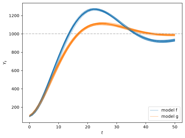
Now let’s simulate two Samuelson models with different accelerator coefficients and plot their sample paths
Both models have the same steady state \(Y^* = 20/(1 - 0.98) = 1000\).
Both start from \(Y_0 \sim \mathcal{N}(100, 25)\) and \(Y_{-1} \sim \mathcal{N}(95, 25)\), far below \(Y^*\).
# Model f: Higher accelerator coefficient
a_f, b_f = 0.98, 0.9
γ_f, G_f, σ_f = 10, 10, 0.5

# Model g: Lower accelerator coefficient
a_g, b_g = 0.98, 0.85
γ_g, G_g, σ_g = 10, 10, 0.5


model_sam_f, G_obs_f, info_f = create_samuelson_var_model(
    a_f, b_f, γ_f, G_f, σ_f,
    stationary_init=False,
    y_0=100, y_m1=95
)

model_sam_g, G_obs_g, info_g = create_samuelson_var_model(
    a_g, b_g, γ_g, G_g, σ_g,
    stationary_init=False,
    y_0=100, y_m1=95
)

T = 50
N_paths = 50

# Get both states and observables
states_f, obs_f = simulate_samuelson(model_sam_f, G_obs_f, T, rng, N_paths)
states_g, obs_g = simulate_samuelson(model_sam_g, G_obs_g, T, rng, N_paths)

output_paths_f = obs_f[:, :, 0]
output_paths_g = obs_g[:, :, 0]

print("model f:")
print(f"  ρ_1 = a + b = {info_f['ρ_1']:.2f}")
print(f"  ρ_2 = -b = {info_f['ρ_2']:.2f}")
print(f"  roots: {info_f['roots']}")
print(f"  dynamics: {info_f['dynamics']}")
print(f"  steady state: {info_f['steady_state']:.1f}")

print("\nmodel g:")
print(f"  ρ_1 = a + b = {info_g['ρ_1']:.2f}")
print(f"  ρ_2 = -b = {info_g['ρ_2']:.2f}")
print(f"  roots: {info_g['roots']}")
print(f"  dynamics: {info_g['dynamics']}")
print(f"  steady state: {info_g['steady_state']:.1f}")


fig, ax = plt.subplots(1, 1)

for i in range(min(20, N_paths)):
    ax.plot(output_paths_f[i], alpha=0.6, color='C0', linewidth=0.8)
    ax.plot(output_paths_g[i], alpha=0.6, color='C1', linewidth=0.8)
ax.axhline(info_f['steady_state'], color='gray', linestyle='--', alpha=0.5)
ax.set_xlabel('$t$')
ax.set_ylabel('$Y_t$')
ax.legend(['model f', 'model g'], loc='lower right')
plt.tight_layout()
plt.show()
model f:
  ρ_1 = a + b = 1.88
  ρ_2 = -b = -0.90
  roots: [0.94+0.12806248j 0.94-0.12806248j]
  dynamics: Damped oscillations
  steady state: 1000.0

model g:
  ρ_1 = a + b = 1.83
  ρ_2 = -b = -0.85
  roots: [0.915+0.11302655j 0.915-0.11302655j]
  dynamics: Damped oscillations
  steady state: 1000.0
# Compute likelihood ratios
L_ratios_ff = compute_likelihood_ratio_var(states_f, model_sam_f, model_sam_g)
L_ratios_gf = compute_likelihood_ratio_var(states_g, model_sam_f, model_sam_g)

fig, axes = plt.subplots(1, 2, figsize=(12, 5))

ax = axes[0]
for i in range(min(20, N_paths)):
    ax.plot(L_ratios_ff[i], alpha=0.5, color='C0', lw=0.8)
ax.axhline(y=0, color='gray', linestyle='--', alpha=0.5)
ax.set_title(r'$\log L_t$ (nature = f)')
ax.set_ylabel(r'$\log L_t$')

ax = axes[1]
for i in range(min(20, N_paths)):
    ax.plot(L_ratios_gf[i], alpha=0.5, color='C1', lw=0.8)
ax.axhline(y=0, color='gray', linestyle='--', alpha=0.5)
ax.set_title(r'$\log L_t$ (nature = g)')
plt.show()
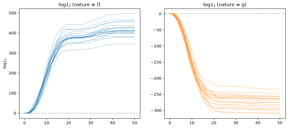
In the figure on the left, data are generated by \(f\) and the log likelihood ratio diverges to plus infinity.
In the figure on the right, data are generated by \(g\) and the log likelihood ratio diverges to negative infinity.
In both cases, the likelihood ratio processes eventually lead us to select the correct model.
Almost all of the information that discriminates between the two models comes from the transient that carries \(Y_t\) from \(Y_0 \approx 100\) toward \(Y^* = 1000\).
The two models share \(a\), \(\gamma\), \(G\), \(\sigma\), and \(Y^*\); they differ only in the accelerator coefficient \(b\).
Their forecasts of \(Y_{t+1}\) differ by \((b_f - b_g)(Y_t - Y_{t-1}) = 0.05 \, \Delta Y_t\).
Because the two models share \(\sigma\), the expected increment of \(\log L_t\) under \(f\) is
and \(E_g [-\ell_{t+1} | x_t]\) is given by the same formula.
Along the transient, \(|\Delta Y_t|\) is large relative to \(\sigma = 0.5\).
In the stationary distribution, \(\Delta Y_t\) is small, and the KL divergence rate is \(h_{KL}(f, g) = (b_f - b_g)^2 E_f[(\Delta Y_t)^2] / (2\sigma^2)\).
The function below computes this rate from the stationary distribution of \(x_t\) for a model created with stationary_init=True.
def samuelson_kl_rate(model_f, model_g):
    """
    KL divergence rate h_KL(f, g) for two Samuelson models created with
    stationary_init=True; only the Y component of x_{t+1} is random
    """
    σ2_f, σ2_g = model_f.CC[1, 1], model_g.CC[1, 1]
    d = model_f.A[1] - model_g.A[1]      # difference in forecasts of Y_{t+1}
    M_f = model_f.Σ_0 + np.outer(model_f.μ_0, model_f.μ_0)   # E_f[x_t x_t']
    return 0.5 * (σ2_f / σ2_g - 1 + np.log(σ2_g / σ2_f)
                  + d @ M_f @ d / σ2_g)

model_stat_f, _, _ = create_samuelson_var_model(
    a_f, b_f, γ_f, G_f, σ_f, stationary_init=True)
model_stat_g, _, _ = create_samuelson_var_model(
    a_g, b_g, γ_g, G_g, σ_g, stationary_init=True)

h_fg = samuelson_kl_rate(model_stat_f, model_stat_g)
h_gf = samuelson_kl_rate(model_stat_g, model_stat_f)

print(f"median log L_{T}: nature = f: {np.median(L_ratios_ff[:, -1]):.1f}, "
      f"nature = g: {np.median(L_ratios_gf[:, -1]):.1f}")
print(f"stationary sd of ΔY_t under f: "
      f"{np.sqrt(2 * (model_stat_f.Σ_0[1, 1] - model_stat_f.Σ_0[1, 2])):.2f}")
print(f"h_KL(f, g) = {h_fg:.4f}, h_KL(g, f) = {h_gf:.4f}")
print(f"{T} × h_KL(f, g) = {T * h_fg:.2f}, {T} × h_KL(g, f) = {T * h_gf:.2f}")

# Expected increments E[ℓ_t | x_{t-1}] along the simulated paths
d = model_sam_f.A[1] - model_sam_g.A[1]
σ2 = σ_f**2
inc_f = ((states_f[:, :-1, :] @ d)**2 / (2 * σ2)).mean(axis=0)
inc_g = ((states_g[:, :-1, :] @ d)**2 / (2 * σ2)).mean(axis=0)
t_grid = np.arange(1, T + 1)

print(f"largest mean expected increment: "
      f"nature = f: {inc_f.max():.1f} at t = {t_grid[inc_f.argmax()]}, "
      f"nature = g: {inc_g.max():.1f} at t = {t_grid[inc_g.argmax()]}")

fig, ax = plt.subplots()
ax.semilogy(t_grid, inc_f, color='C0', lw=2,
            label=r'$E_f[\ell_t | x_{t-1}]$, mean over paths')
ax.semilogy(t_grid, inc_g, color='C1', lw=2,
            label=r'$E_g[-\ell_t | x_{t-1}]$, mean over paths')
ax.axhline(h_fg, color='C0', ls='--', lw=2, label=r'$h_{KL}(f, g)$')
ax.axhline(h_gf, color='C1', ls='--', lw=2, label=r'$h_{KL}(g, f)$')
ax.set_xlabel('$t$')
ax.set_ylabel('expected increment')
ax.legend()
plt.show()
median log L_50: nature = f: 413.5, nature = g: -279.2
stationary sd of ΔY_t under f: 1.15
h_KL(f, g) = 0.0066, h_KL(g, f) = 0.0045
50 × h_KL(f, g) = 0.33, 50 × h_KL(g, f) = 0.23
largest mean expected increment: nature = f: 33.8 at t = 10, nature = g: 23.9 at t = 9
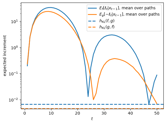
The expected increments reach about \(34\) under \(f\) and \(24\) under \(g\) near \(t = 10\), when \(Y_t\) rises fastest.
They approach the stationary rates \(h_{KL}(f, g)\) and \(h_{KL}(g, f)\) only near the turning points of the oscillation, where \(\Delta Y_t\) is close to zero.
The stationary standard deviation of \(\Delta Y_t\) under \(f\) is \(1.15\).
From the stationary distribution, \(50\) periods raise \(E_f [\log L_t]\) by only about \(0.33\), while the transient raises the median of \(\log L_{50}\) to about \(400\).
Exercise Exercise 24.2 starts both models from their stationary distributions and studies how much harder the two models are to tell apart.
24.8. Exercises#
Exercise 24.1
Derive formula (24.4) for the KL divergence rate \(h_{KL}(f, g)\).
Use the formula for the Kullback–Leibler divergence of two multivariate normal distributions:
Then verify by simulation that \(\frac{1}{t} \log L_t \to h_{KL}(f, g)\) when \(f\) generates the data and \(\frac{1}{t} \log L_t \to -h_{KL}(g, f)\) when \(g\) generates the data.
Do this for Examples 1 and 2 with \(T = 2000\).
Solution
Under model \(f\), \(x_t | x_{t-1} \sim \mathcal{N}(A_f x_{t-1}, \Sigma_f)\); under model \(g\), \(x_t | x_{t-1} \sim \mathcal{N}(A_g x_{t-1}, \Sigma_g)\).
So \(E_f [\ell_t | x_{t-1}] = KL\bigl(\mathcal{N}(A_f x_{t-1}, \Sigma_f), \mathcal{N}(A_g x_{t-1}, \Sigma_g)\bigr)\).
Setting \(\mu_1 - \mu_2 = (A_f - A_g) x_{t-1}\) in the formula above gives
Under \(f\), \(x_{t-1} \sim \mathcal{N}(0, V_f)\).
For any matrix \(M\), \(E [x_{t-1}^\top M x_{t-1}] = \operatorname{tr}(M V_f)\).
With \(M = (A_f - A_g)^\top \Sigma_g^{-1} (A_f - A_g)\) and the cyclic property of the trace,
Taking expectations of \(E_f [\ell_t | x_{t-1}]\) over \(x_{t-1}\) gives (24.4).
Because \(x_{t-1}\) has the same distribution \(\mathcal{N}(0, V_f)\) for every \(t\), every increment \(\ell_t\) has mean \(h_{KL}(f, g)\) and
The ergodic theorem implies \(\frac{1}{t} \sum_{s=1}^t \ell_s \to h_{KL}(f, g)\) almost surely, and \(\frac{1}{t} \log \frac{p_f(x_0)}{p_g(x_0)} \to 0\).
Here is the simulation.
T_long = 2000
N_long = 20
t_grid = np.arange(1, T_long + 1)

fig, axes = plt.subplots(1, 2, figsize=(12, 5))

for ax, (name, m_f, m_g) in zip(axes, examples):
    for nature, m_true, rate, color in [
            ('f', m_f, kl_rate_var(m_f, m_g), 'C0'),
            ('g', m_g, -kl_rate_var(m_g, m_f), 'C1')]:
        paths = simulate_var(m_true, T_long, rng, N_long)
        log_L = compute_likelihood_ratio_var(paths, m_f, m_g)
        avg = log_L[:, 1:] / t_grid
        ax.plot(t_grid, avg.T, color=color, alpha=0.2, lw=1)
        ax.axhline(rate, color=color, ls='--', lw=2,
                   label=f'theory (nature = {nature})')
        print(f"{name}, nature = {nature}: mean of log L_T / T = "
              f"{avg[:, -1].mean():.4f}, theory = {rate:.4f}")
    ax.set_xscale('log')
    ax.set_xlabel('$t$')
    ax.set_ylabel(r'$\log L_t / t$')
    ax.set_title(name)
    ax.legend()

plt.tight_layout()
plt.show()
Example 1, nature = f: mean of log L_T / T = 0.1420, theory = 0.1392
Example 1, nature = g: mean of log L_T / T = -0.2068, theory = -0.2079
Example 2, nature = f: mean of log L_T / T = 0.3423, theory = 0.3443
Example 2, nature = g: mean of log L_T / T = -0.9629, theory = -0.9614
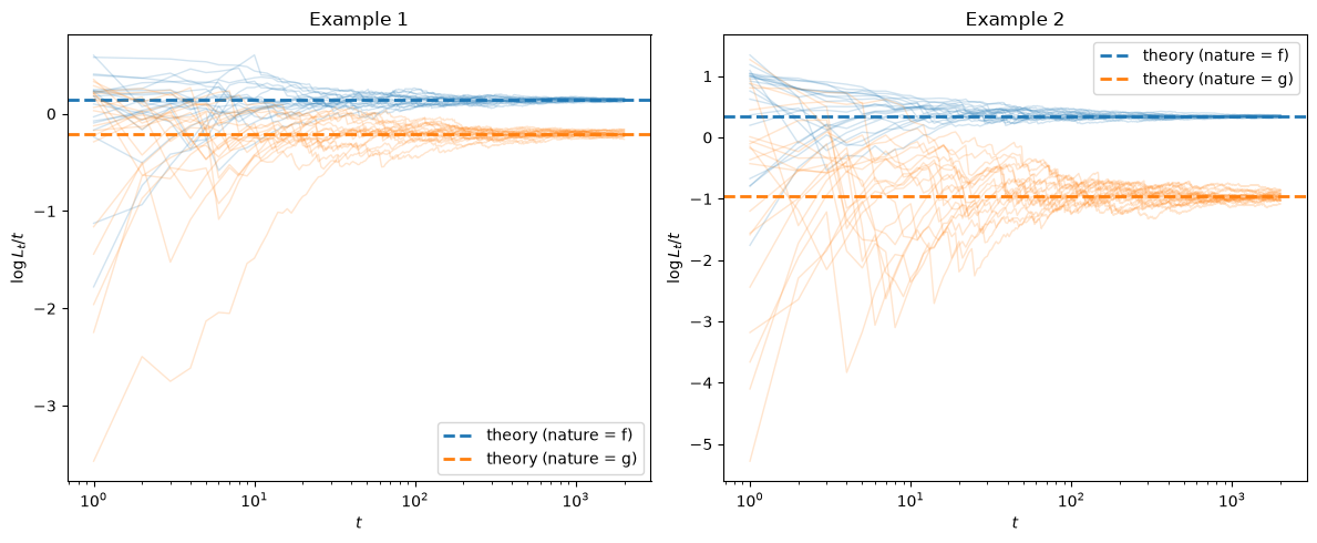
In all four cases, \(\frac{1}{t} \log L_t\) settles down near the theoretical rate.
Exercise 24.2
In the Samuelson example, both models start from \(Y_0 \approx 100\), far below the common steady state \(Y^* = 1000\).
Start both models from their stationary distributions instead by using the models model_stat_f and model_stat_g created with stationary_init=True.
Simulate 500 paths of length \(T = 50\) from each model. Report the median of \(\log L_{50}\) and the error probabilities \(\alpha_{50}\), \(\beta_{50}\), and \(\frac{1}{2}(\alpha_{50} + \beta_{50})\). Compare them with those for the paths that start from \(Y_0 \approx 100\).
Use
samuelson_kl_rateand the Kullback–Leibler divergence of the two stationary distributions of \((Y_0, Y_{-1})\) to compute the number of periods \(t\) at which \(E_f [\log L_t] = 5\).Simulate paths of that length and plot \(\alpha_t\) and \(\beta_t\).
Solution
Here are the error probabilities at \(T = 50\) for the two initial conditions.
T_s, N_s = 50, 500

paths_stat_f = simulate_var(model_stat_f, T_s, rng, N_s)
paths_stat_g = simulate_var(model_stat_g, T_s, rng, N_s)
log_L_stat_f = compute_likelihood_ratio_var(paths_stat_f,
                                            model_stat_f, model_stat_g)
log_L_stat_g = compute_likelihood_ratio_var(paths_stat_g,
                                            model_stat_f, model_stat_g)

for label, log_L_f, log_L_g in [
        ("stationary start", log_L_stat_f, log_L_stat_g),
        ("Y_0 ≈ 100", L_ratios_ff, L_ratios_gf)]:
    α = np.mean(log_L_f[:, -1] < 0)
    β = np.mean(log_L_g[:, -1] >= 0)
    print(f"{label}:")
    print(f"  median log L_50: nature = f: {np.median(log_L_f[:, -1]):.3f}, "
          f"nature = g: {np.median(log_L_g[:, -1]):.3f}")
    print(f"  α_50 = {α:.3f}, β_50 = {β:.3f}, "
          f"average error = {0.5 * (α + β):.3f}")
stationary start:
  median log L_50: nature = f: 0.132, nature = g: -0.452
  α_50 = 0.426, β_50 = 0.244, average error = 0.335
Y_0 ≈ 100:
  median log L_50: nature = f: 413.526, nature = g: -279.175
  α_50 = 0.000, β_50 = 0.000, average error = 0.000
From the stationary distributions, the medians of \(\log L_{50}\) are within \(0.5\) of zero, \(\alpha_{50}\) is about \(0.4\), and the likelihood ratio test selects the wrong model in about a third of the samples.
From \(Y_0 \approx 100\), it selects the correct model in all \(50\) samples from each model.
Under \(f\), \(E_f [\log L_t] = KL_0 + t \, h_{KL}(f, g)\), where \(KL_0\) is the Kullback–Leibler divergence of the stationary distribution of \((Y_0, Y_{-1})\) under \(g\) from that under \(f\).
def kl_gauss(μ_1, Σ_1, μ_2, Σ_2):
    """
    KL divergence of N(μ_2, Σ_2) from N(μ_1, Σ_1)
    """
    n = len(μ_1)
    Σ_2_inv = np.linalg.inv(Σ_2)
    d = μ_1 - μ_2
    return 0.5 * (np.trace(Σ_2_inv @ Σ_1) - n + d @ Σ_2_inv @ d
                  + np.log(np.linalg.det(Σ_2) / np.linalg.det(Σ_1)))

KL_0 = kl_gauss(model_stat_f.μ_0[1:], model_stat_f.Σ_0[1:, 1:],
                model_stat_g.μ_0[1:], model_stat_g.Σ_0[1:, 1:])
t_star = int(np.ceil((5 - KL_0) / h_fg))

print(f"KL_0 = {KL_0:.4f}, h_KL(f, g) = {h_fg:.5f}")
print(f"E_f[log L_50]: theory = {KL_0 + 50 * h_fg:.3f}, "
      f"simulation = {log_L_stat_f[:, -1].mean():.3f}")
print(f"stationary start: E_f[log L_t] = 5 at t = {t_star}")

# Transient from Y_0 ≈ 100: cumulative mean expected increments
t_transient = np.argmax(np.cumsum(inc_f) >= 5) + 1
print(f"Y_0 ≈ 100: cumulative expected increments reach 5 at t = {t_transient}")
KL_0 = 0.0881, h_KL(f, g) = 0.00661
E_f[log L_50]: theory = 0.419, simulation = 0.391
stationary start: E_f[log L_t] = 5 at t = 743
Y_0 ≈ 100: cumulative expected increments reach 5 at t = 3
About \(750\) periods of stationary data contain as much information about \(b\), on average, as the first three periods of the transient from \(Y_0 \approx 100\).
N_star = 200

paths_f = simulate_var(model_stat_f, t_star, rng, N_star)
paths_g = simulate_var(model_stat_g, t_star, rng, N_star)
log_L_f = compute_likelihood_ratio_var(paths_f, model_stat_f, model_stat_g)
log_L_g = compute_likelihood_ratio_var(paths_g, model_stat_f, model_stat_g)

α_t = np.mean(log_L_f < 0, axis=0)
β_t = np.mean(log_L_g >= 0, axis=0)

fig, ax = plt.subplots()
ax.plot(α_t, color='C0', lw=2, label=r'$\alpha_t$')
ax.plot(β_t, color='C1', lw=2, label=r'$\beta_t$')
ax.plot(0.5 * (α_t + β_t), 'g--', lw=2, label='average error')
ax.set_xlabel('$t$')
ax.set_ylabel('error probability')
ax.legend()
plt.show()

print(f"at t = {t_star}: α = {α_t[-1]:.3f}, β = {β_t[-1]:.3f}")
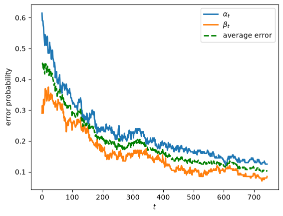
at t = 743: α = 0.125, β = 0.085
Even after about \(750\) periods, both error probabilities remain roughly \(0.1\).
Exercise 24.3
Suppose that neither \(f\) nor \(g\) of Example 2 generates the data.
Instead a third VAR \(h\) with matrices \((A_h, C_h)\) generates the data.
Show that
almost surely, where \(h_{KL}(h, \cdot)\) is (24.4) with \(h\) in place of \(f\).
This is the VAR counterpart of the formula in A helpful formula of Likelihood Ratio Processes.
Verify the limit by simulation for \((A_h, C_h) = (A_f, C_g)\) and for \((A_h, C_h) = (A_g, C_f)\).
Which model does the likelihood ratio select in each case?
Solution
Write
Taking expectations under \(h\), with \(x_{t-1}\) drawn from the stationary distribution of \(h\), gives \(E_h [\ell_t] = h_{KL}(h, g) - h_{KL}(h, f)\).
The ergodic theorem under \(h\) then gives the almost sure limit.
model_h1 = create_var_model(model2_f.A, model2_g.C)
model_h2 = create_var_model(model2_g.A, model2_f.C)

T_h, N_h = 1000, 20
t_grid = np.arange(1, T_h + 1)

fig, axes = plt.subplots(1, 2, figsize=(12, 5))

cases = [("(A_f, C_g)", r'$(A_h, C_h) = (A_f, C_g)$', model_h1),
         ("(A_g, C_f)", r'$(A_h, C_h) = (A_g, C_f)$', model_h2)]

for ax, (name, title, m_h) in zip(axes, cases):
    K_f = kl_rate_var(m_h, model2_f)
    K_g = kl_rate_var(m_h, model2_g)
    paths = simulate_var(m_h, T_h, rng, N_h)
    log_L = compute_likelihood_ratio_var(paths, model2_f, model2_g)
    avg = log_L[:, 1:] / t_grid
    ax.plot(t_grid, avg.T, color='C2', alpha=0.3, lw=1)
    ax.axhline(K_g - K_f, color='k', ls='--', lw=2,
               label=r'$h_{KL}(h, g) - h_{KL}(h, f)$')
    ax.set_xscale('log')
    ax.set_xlabel('$t$')
    ax.set_ylabel(r'$\log L_t / t$')
    ax.set_title(title)
    ax.legend()
    print(f"(A_h, C_h) = {name}: h_KL(h, f) = {K_f:.4f}, "
          f"h_KL(h, g) = {K_g:.4f}, difference = {K_g - K_f:.4f}, "
          f"mean of log L_T / T = {avg[:, -1].mean():.4f}")

plt.tight_layout()
plt.show()
(A_h, C_h) = (A_f, C_g): h_KL(h, f) = 0.8069, h_KL(h, g) = 0.0586, difference = -0.7482, mean of log L_T / T = -0.7711
(A_h, C_h) = (A_g, C_f): h_KL(h, f) = 0.0542, h_KL(h, g) = 0.3181, difference = 0.2639, mean of log L_T / T = 0.2643
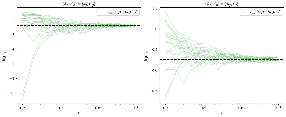
When \((A_h, C_h) = (A_f, C_g)\), \(\log L_t \to -\infty\) and the likelihood ratio selects \(g\), although \(f\) has the correct transition matrix.
When \((A_h, C_h) = (A_g, C_f)\), \(\log L_t \to +\infty\) and the likelihood ratio selects \(f\), although \(g\) has the correct transition matrix.
In both cases the likelihood ratio selects the model with the correct shock covariance matrix.
When \((A_h, C_h) = (A_f, C_g)\), \(h_{KL}(h, f)\) consists only of covariance terms and \(h_{KL}(h, g)\) only of a conditional-mean term.
When \((A_h, C_h) = (A_g, C_f)\), the roles of \(f\) and \(g\) are reversed.
In both cases the covariance terms are larger, as in the decomposition for Example 2 above.