34. Merging of Opinions: The Blackwell–Dubins Theorem#
34.1. Overview#
This lecture studies the merging-of-opinions theorem of Blackwell and Dubins [1962].
The theorem asks a simple question:
If two agents hold different prior beliefs about a stochastic process but observe the same stream of data indefinitely, will their probability assessments eventually converge?
The answer is yes under an absolute-continuity condition.
If \(Q \ll P\) (that is, \(P\) dominates \(Q\)), then the conditional distributions under \(P\) and \(Q\) over the entire future path merge in total variation, \(Q\)-almost surely.
If in addition \(P \ll Q\) (so that \(P \sim Q\)), then the same conclusion holds under both agents’ probabilities.
This result connects to several other ideas:
Bayesian consistency: posterior predictions approach the truth when the prior lies in the right absolute-continuity class (Likelihood Ratio Processes and Bayesian Learning).
Agreement results: Aumann [1976] studies agents with a common prior and private information; Blackwell–Dubins studies agents with different priors and common information.
Kakutani’s dichotomy: for product measures, equivalence versus singularity can be read from a Hellinger criterion.
We develop the theory in discrete time and then sketch the continuous-time analogue.
Throughout, we use the Beta–Bernoulli model as a running example.
Two agents observe the same stream of coin flips but start from different priors over the coin’s bias.
Let us start with some imports.
import numpy as np
import matplotlib.pyplot as plt
from scipy.stats import beta as beta_dist, binom, betabinom, norm
from scipy.special import betaln, beta as beta_fn, polygamma
34.2. Probability measures on sequence spaces#
34.2.1. The sequence space and its filtration#
Let \((S, \mathscr{S})\) be a standard Borel space (i.e., a measurable space isomorphic to a Borel subset of a complete separable metric space), called the signal space.
The standard Borel assumption guarantees the existence of regular conditional distributions, which the theorem requires.
Set \(\Omega = S^{\mathbb{N}}\), the set of all infinite sequences \(\omega = (x_1, x_2, \ldots)\) with \(x_n \in S\), equipped with the product \(\sigma\)-algebra \(\mathscr{F} = \mathscr{S}^{\otimes \mathbb{N}}\).
For each \(n \geq 1\), define the finite-horizon \(\sigma\)-algebra
and set \(\mathscr{F}_0 = \{\emptyset, \Omega\}\), so \(\mathscr{F}_0 \subseteq \mathscr{F}_1 \subseteq \mathscr{F}_2 \subseteq \cdots \subseteq \mathscr{F}\).
Define \(\mathscr{F}_\infty = \sigma\!\left(\bigcup_{n \geq 1} \mathscr{F}_n\right)\), the \(\sigma\)-algebra of events that can eventually be learned.
Cylinder sets \(\{x_1 \in A_1, \ldots, x_n \in A_n\}\) generate the product \(\sigma\)-algebra and belong to \(\bigcup_n \mathscr{F}_n\), so \(\mathscr{F}_\infty = \mathscr{F}\).
The \(\sigma\)-algebra \(\mathscr{F}_\infty\) differs from the tail \(\sigma\)-algebra \(\mathscr{T} = \bigcap_{n \geq 1} \sigma(x_n, x_{n+1}, \ldots)\), whose events, such as \(\{x_n \in A \text{ for infinitely many } n\}\), do not depend on any finite stretch of data.
The collection \(\{\mathscr{F}_n\}_{n \geq 1}\) is the natural filtration generated by the observation process; \(\mathscr{F}_n\) encodes everything that can be learned from the first \(n\) data points.
Let \(P\) and \(Q\) denote two probability measures on \((\Omega, \mathscr{F})\).
Write \(P_n = P|_{\mathscr{F}_n}\) and \(Q_n = Q|_{\mathscr{F}_n}\) for their restrictions to the history up to time \(n\).
34.2.2. Absolute continuity#
Definition 34.1 (Absolute Continuity)
\(P\) is absolutely continuous with respect to \(Q\), written \(P \ll Q\), if \(Q(A) = 0\) implies \(P(A) = 0\) for every \(A \in \mathscr{F}\).
They are mutually absolutely continuous, or equivalent, written \(P \sim Q\), if both \(P \ll Q\) and \(Q \ll P\).
\(P\) is locally absolutely continuous with respect to \(Q\) if \(P_n \ll Q_n\) for every \(n \geq 1\).
Global absolute continuity \(P \ll Q\) implies local absolute continuity, but not conversely.
Mutual absolute continuity means the two agents agree on which events are possible.
They can disagree about probabilities, but neither agent rules out an event the other deems possible.
34.2.3. Total variation distance#
Definition 34.2 (Total Variation Distance)
For two probability measures \(\mu\) and \(\nu\) on \((E, \mathscr{E})\),
where \(\lambda\) is any dominating measure, meaning \(\mu \ll \lambda\) and \(\nu \ll \lambda\) (for example, \(\lambda = \mu + \nu\)).
The distance \(\|\mu - \nu\|_{\mathrm{TV}}\) lies in \([0,1]\); it equals 0 if and only if \(\mu = \nu\) and 1 if and only if \(\mu \perp \nu\) (mutual singularity).
When \(\mu \ll \nu\) with \(f = d\mu/d\nu\),
Exercise 34.1
Show the identity above.
Hint: Start from \(\|\mu - \nu\|_{\mathrm{TV}} = \tfrac{1}{2}\,\mathbb{E}_\nu[|f - 1|]\) (which follows from taking \(\nu\) as the dominating measure) and use the fact that \(\mathbb{E}_\nu[f] = 1\).
Solution
Since \(\mu \ll \nu\), we can use \(\nu\) as the dominating measure, so \(d\mu/d\nu = f\) and \(d\nu/d\nu = 1\), giving
Write \(|f-1| = (f-1)^+ + (1-f)^+\).
Since \(\mu\) is a probability measure, \(\mathbb{E}_\nu[f] = 1\), so the two parts contribute equally: \(\mathbb{E}_\nu[(f-1)^+] = \mathbb{E}_\nu[(1-f)^+]\).
Therefore \(\tfrac{1}{2}\,\mathbb{E}_\nu[|f-1|] = \mathbb{E}_\nu[(f-1)^+]\).
Next, note that \((f-1)^+ = f - \min(f,1)\), so \(\mathbb{E}_\nu[(f-1)^+] = \mathbb{E}_\nu[f] - \mathbb{E}_\nu[\min(f,1)] = 1 - \mathbb{E}_\nu[\min(f,1)]\).
Total variation is one of the strongest standard notions of distance between probability measures.
If two measures are close in total variation, then their probabilities of every event are close.
34.2.4. The merging question#
The Blackwell–Dubins theorem studies the conditional distribution of the future given the past.
At time \(n\), after observing \((x_1,\ldots,x_n)\), each agent forms a conditional distribution over all future events:
These are probability measures on the whole future path, not just the next observation.
The merging question asks whether
almost surely as \(n \to \infty\).
At \(n = 0\) the conditioning is trivial and \(d_0 = \|P - Q\|_{\mathrm{TV}}\).
34.3. The likelihood-ratio martingale#
Our main tool is the Radon–Nikodym derivative process.
34.3.1. The likelihood ratio#
Since \(Q \ll P\) implies \(Q_n \ll P_n\) for every \(n\), the Radon–Nikodym theorem guarantees the existence of the likelihood ratio
The key structural property is that global absolute continuity \(Q \ll P\) implies the existence of an overall Radon–Nikodym derivative \(Z = dQ/dP\) on all of \((\Omega, \mathscr{F})\), and
That is, \(\{Z_n, \mathscr{F}_n\}_{n \geq 0}\) is a non-negative, uniformly integrable \(P\)-martingale with \(Z_0 = 1\).
Throughout the lecture, \(Z\) and \(Z_n\) denote densities of \(Q\) with respect to \(P\).
Posterior probabilities are martingales of the same kind; Blackwell’s Theorem on Comparing Experiments uses that property to compare experiments.
Lemma 34.1 (Martingale Convergence)
The likelihood-ratio process \(\{Z_n\}\) satisfies:
\(Z_n \to Z_\infty\) \(P\)-almost surely as \(n \to \infty\).
\(Z_\infty = \mathbb{E}_P[Z \,|\, \mathscr{F}_\infty] = Z\) \(P\)-a.s.
\(Z_n \to Z_\infty\) in \(L^1(P)\): \(\;\mathbb{E}_P[|Z_n - Z_\infty|] \to 0\).
Proof sketch. Non-negativity and the martingale property give boundedness in \(L^1(P)\).
Then almost-sure convergence follows from Doob’s martingale convergence theorem [Doob, 1953].
Uniform integrability (which follows from \(Z \in L^1(P)\) via the conditional Jensen inequality) upgrades this to \(L^1(P)\) convergence.
Lévy’s upward theorem identifies the limit as \(\mathbb{E}_P[Z \,|\, \mathscr{F}_\infty]\), which equals \(Z\) because \(\mathscr{F}_\infty = \mathscr{F}\). \(\square\)
From here on we write \(Z_\infty\) for \(Z = dQ/dP\).
34.3.2. Connecting conditional measures to the likelihood ratio#
The following identity connects the likelihood ratio to the conditional distributions.
On the set \(\{Z_n > 0\}\), the Radon–Nikodym derivative of \(Q(\,\cdot\,|\,\mathscr{F}_n)\) with respect to \(P(\,\cdot\,|\,\mathscr{F}_n)\) is
This is the abstract Bayes formula \(Q(A \,|\, \mathscr{F}_n) = \mathbb{E}_P[Z_\infty \mathbf{1}_A \,|\, \mathscr{F}_n] / \mathbb{E}_P[Z_\infty \,|\, \mathscr{F}_n]\).
The set \(\{Z_n > 0\}\) has \(Q\)-probability one, because \(Q(Z_n = 0) = \mathbb{E}_P[Z_n \mathbf{1}\{Z_n = 0\}] = 0\).
Applying the total-variation formula with \(f = Z_\infty / Z_n\) then gives
Because \(Z_n\) is \(\mathscr{F}_n\)-measurable, the same quantity is a ratio of conditional expectations:
The second equality holds because \(\mathbb{E}_P[Z_\infty - Z_n \,|\, \mathscr{F}_n] = 0\), so the positive and negative parts of \(Z_\infty - Z_n\) have equal conditional means.
Multiplying through by \(Z_n\) and taking the \(P\)-expectation (then using \(\mathbb{E}_P[Z_n \, g] = \mathbb{E}_Q[g]\) for non-negative \(\mathscr{F}_n\)-measurable \(g\)):
So the \(L^1(P)\) convergence of the martingale gives \(\mathbb{E}_Q[d_n] \to 0\), and its rate governs how fast \(\mathbb{E}_Q[d_n]\) goes to zero.
34.4. The Blackwell–Dubins theorem#
Theorem 34.1 (Blackwell–Dubins (1962))
Let \(P\) and \(Q\) be probability measures on \((\Omega, \mathscr{F})\) with \(Q \ll P\).
Define
Then \(d_n \to 0\) \(Q\)-almost surely.
The identity \(\mathbb{E}_Q[d_n] = \tfrac{1}{2}\,\mathbb{E}_P[|Z_\infty - Z_n|] \to 0\) gives convergence in \(Q\)-probability.
The proof of almost-sure convergence has three steps.
Step 1. A formula for \(d_n\).
Equation (34.1) writes \(d_n\) as the ratio of \(\mathbb{E}_P[|Z_\infty - Z_n| \,|\, \mathscr{F}_n]\) to \(2 Z_n\), \(Q\)-a.s.
Step 2. The denominator converges to a positive limit.
By Lemma 34.1, \(Z_n \to Z_\infty\) \(P\)-a.s., hence \(Q\)-a.s. because \(Q \ll P\).
The limit is positive \(Q\)-a.s., because \(Q(Z_\infty = 0) = \mathbb{E}_P[Z_\infty \mathbf{1}\{Z_\infty = 0\}] = 0\).
Step 3. The numerator converges to zero.
Fix \(M > 0\) and split \(Z_\infty = U + V\), where \(U = \min(Z_\infty, M)\) and \(V = (Z_\infty - M)^+\).
Let \(U_n = \mathbb{E}_P[U \,|\, \mathscr{F}_n]\) and \(V_n = \mathbb{E}_P[V \,|\, \mathscr{F}_n]\), so \(Z_n = U_n + V_n\).
The triangle inequality gives \(|Z_\infty - Z_n| \leq |U - U_n| + V + V_n\), and conditioning on \(\mathscr{F}_n\) gives
Lévy’s upward theorem gives \(V_n \to V\) \(P\)-a.s.
For the bounded part, fix \(m\) and let \(W_m = \sup_{k \geq m} |U - U_k| \leq 2M\).
For \(n \geq m\), \(\mathbb{E}_P[|U - U_n| \,|\, \mathscr{F}_n] \leq \mathbb{E}_P[W_m \,|\, \mathscr{F}_n]\), and Lévy’s upward theorem sends the right side to \(W_m\) as \(n \to \infty\).
Lévy’s upward theorem also gives \(U_k \to U\) \(P\)-a.s., so \(W_m \to 0\) as \(m \to \infty\).
Combining these limits,
for every \(M\).
Letting \(M \to \infty\) through the integers sends the right side to zero, because \(Z_\infty\) is finite.
So the numerator converges to zero \(P\)-a.s., hence \(Q\)-a.s.
Steps 1–3 give \(d_n \to 0\) \(Q\)-a.s. \(\square\)
The argument for the bounded part \(U\) is Hunt’s lemma.
The proof uses no monotonicity of \(\{d_n\}\); a later section shows that \(\{d_n\}\) need not be a supermartingale.
Remark 34.1 (One-Sided vs. Mutual Absolute Continuity)
The theorem requires only \(Q \ll P\), not \(P \ll Q\).
One-sided absolute continuity \(Q \ll P\) gives merging \(Q\)-almost surely.
Since \(Q \ll P\) means every \(P\)-null set is also \(Q\)-null, \(Q\)-a.s. convergence does not automatically imply \(P\)-a.s. convergence.
To conclude that \(d_n \to 0\) under both agents’ measures, one needs mutual absolute continuity \(P \sim Q\).
With \(P \ll Q\) added, the proof can be run with the roles of \(P\) and \(Q\) swapped, yielding \(d_n \to 0\) \(P\)-a.s. as well.
Remark 34.2 (Sharpness)
Absolute continuity matters.
When \(P\) and \(Q\) are singular, merging can fail completely.
Suppose \(P \perp Q\) and \(P_n \sim Q_n\) for every \(n\).
Take \(S \in \mathscr{F}\) with \(P(S) = 1\) and \(Q(S) = 0\).
Then \(P(S \,|\, \mathscr{F}_n) = 1\) \(P\)-a.s. and \(Q(S \,|\, \mathscr{F}_n) = 0\) \(Q\)-a.s.
The events \(\{P(S \,|\, \mathscr{F}_n) = 1\}\) and \(\{Q(S \,|\, \mathscr{F}_n) = 0\}\) belong to \(\mathscr{F}_n\), so local equivalence makes each hold both \(P\)-a.s. and \(Q\)-a.s.
Hence \(d_n \geq |P(S \,|\, \mathscr{F}_n) - Q(S \,|\, \mathscr{F}_n)| = 1\) for every \(n\), under both measures.
The point-mass example below has \(d_n = 1\) for every \(n\).
For product measures, Kakutani’s theorem later gives a sharp equivalence-versus-singularity dichotomy.
34.5. The Beta–Bernoulli model#
Before turning to Python, we introduce the main example used throughout the simulations.
34.5.1. Model#
Suppose the data stream \((x_1, x_2, \ldots)\) consists of IID Bernoulli draws with unknown probability \(p^* \in (0,1)\).
Agent \(i\) has a Beta prior:
After observing \(n\) draws with \(k\) successes, Bayes’ rule yields the posterior
and the one-step-ahead predictive probability is
By the strong law of large numbers, \(k/n \to p^*\) almost surely, so both \(\hat{p}_1^n\) and \(\hat{p}_2^n\) converge to \(p^*\) regardless of the agents’ initial priors \((\alpha_i, \beta_i)\).
34.5.2. The marginal likelihood and likelihood ratio#
For each fixed value of \(p \in (0,1)\), let \(P_p\) denote the IID Bernoulli\((p)\) probability law on infinite sequences.
Agent \(i\) does not know \(p\).
Instead, agent \(i\) places the prior density \(\pi_i\) on \(p\), which induces a probability measure \(P_i\) on data sequences via
So \(P_i\) is the agent’s marginal probability measure over histories after averaging over uncertainty about \(p\).
In particular, if \(x^n\) is an exact observed history with \(k\) successes, then \(P_i(x^n)\) means the probability that agent \(i\) assigns to that history under this mixture measure.
To compute it, start from the Beta density
Given \(p\), the probability of that ordered history is \(p^k (1-p)^{n-k}\).
Therefore
where \(B(a,b) = \Gamma(a)\Gamma(b)/\Gamma(a+b)\) is the beta function.
This expression is the probability of the ordered history \(x^n\).
It depends on the data only through the count \(k\), so histories with the same number of successes receive the same probability.
The likelihood ratio at time \(n\) is therefore
In the notation of the theorem, \(Q = P_1\) and \(P = P_2\).
The process \(\{Z_n\}\) is a martingale under \(P_2\) (agent 2’s probability) and converges almost surely to a finite positive limit \(Z_\infty\), reflecting the fact that \(P_1 \sim P_2\) for any Beta priors with positive parameters.
The limit has a closed form.
Let \(\bar p = \lim_n k_n/n\), which exists \(P_i\)-a.s. because, conditional on \(p\), the strong law of large numbers applies.
Then
Exercise 34.4 asks for a derivation.
For the priors \(\mathrm{Beta}(1, 8)\) and \(\mathrm{Beta}(8, 1)\) used below, \(\pi_1(p) = 8(1-p)^7\) and \(\pi_2(p) = 8p^7\), so
34.5.3. The exact Blackwell–Dubins distance#
For the Beta–Bernoulli model, there is a clean formula for \(d_n\).
By construction, agent \(i\)’s conditional distribution of the future sequence \((x_{n+1}, x_{n+2}, \ldots)\) given \(x^n\) is a mixture of IID Bernoulli\((p)\) processes, with \(p\) drawn from agent \(i\)’s posterior Beta distribution.
Exchangeability and Bayesian Updating describes de Finetti’s theorem, which delivers such a mixture for every exchangeable process; here the mixture holds by construction.
The Bernoulli\((p)^{\infty}\) measures for different \(p\) are mutually singular, and the limiting frequency \(\bar p\) recovers \(p\).
The map \(\omega \mapsto \bar p\) sends each agent’s conditional distribution of the future to that agent’s posterior, so the TV distance between the conditional distributions is at least the TV distance between the posteriors.
Each conditional distribution is the image of a posterior under the Markov kernel \(p \mapsto \mathrm{Bernoulli}(p)^{\infty}\), so the TV distance between the conditional distributions is at most the TV distance between the posteriors.
Therefore
Both posteriors concentrate around \(k_n/n\) with standard deviations of order \(n^{-1/2}\).
Concentration alone does not deliver \(d_n \to 0\).
Two distributions with standard deviation \(s_n\) have a TV distance that goes to zero only if their means differ by \(o(s_n)\).
When \(\alpha_1 + \beta_1 = \alpha_2 + \beta_2 = 9\), as below, the posterior means differ by \(\delta_n = (\alpha_2 - \alpha_1)/(n + 9) = 7/(n+9)\), which is \(O(1/n)\).
Both posterior standard deviations are approximately \(s_n = \sqrt{\hat p_n (1 - \hat p_n)/n}\), where \(\hat p_n = k_n/n\).
Approximating both posteriors by normal distributions with common standard deviation \(s_n\) and means \(\delta_n\) apart gives
where \(\Phi\) is the standard normal CDF.
At \(\hat p_n = 0.65\) the right side is \(5.85/\sqrt{n}\).
The section on the rate of merging checks this approximation.
When \(\alpha_1 + \beta_1 = \alpha_2 + \beta_2\), the ratio of the two posterior densities is proportional to \(((1-p)/p)^{\beta_1 - \beta_2}\), which is monotone in \(p\).
The two densities cross once, at a point \(x^*\), and \(d_n = |F_1(x^*) - F_2(x^*)|\), where \(F_i\) is agent \(i\)’s posterior CDF.
The following code implements the Beta–Bernoulli updating, predictive probabilities, TV distance, and likelihood-ratio computations described above.
def beta_bernoulli_update(data, a0, b0):
    """
    Sequential Beta-Bernoulli Bayesian updating.
    """
    n = len(data)
    cum_k = np.concatenate([[0], np.cumsum(data)])   # cumulative successes
    ns    = np.arange(n + 1)                          # 0, 1, ..., n
    a_post = a0 + cum_k
    b_post = b0 + (ns - cum_k)
    return a_post, b_post


def predictive_prob(a_post, b_post):
    """One-step-ahead predictive probability P(X=1 | data)."""
    return a_post / (a_post + b_post)


def tv_distance_beta(a1, b1, a2, b2):
    """
    Exact TV distance between Beta(a1, b1) and Beta(a2, b2)
    when a1 + b1 = a2 + b2 and a1 != a2.

    The densities cross once, at x_star, where
    log(x_star / (1 - x_star))
        = (betaln(a2, b2) - betaln(a1, b1)) / (b1 - b2).
    Works elementwise on arrays.
    """
    logit_x = (betaln(a2, b2) - betaln(a1, b1)) / (b1 - b2)
    x_star = 1 / (1 + np.exp(-logit_x))
    return np.abs(beta_dist.cdf(x_star, a1, b1)
                  - beta_dist.cdf(x_star, a2, b2))


def log_likelihood_ratio(data, a1, b1, a2, b2):
    """
    Log likelihood ratio log Z_n = log P1_n(data) - log P2_n(data)
    for every prefix of `data`.

    Returns an array of length len(data) + 1, starting at 0 (before data).
    """
    a1p, b1p = beta_bernoulli_update(data, a1, b1)
    a2p, b2p = beta_bernoulli_update(data, a2, b2)
    log_P1 = betaln(a1p, b1p) - betaln(a1, b1)
    log_P2 = betaln(a2p, b2p) - betaln(a2, b2)
    return log_P1 - log_P2


def run_simulation(p_true, a1, b1, a2, b2, n_steps, seed=0):
    """
    Simulate one realisation of the merging experiment.

    Returns a dict with arrays of length n_steps + 1 (index 0 = prior).
    """
    rng  = np.random.default_rng(seed)
    data = rng.binomial(1, p_true, n_steps)

    a1p, b1p = beta_bernoulli_update(data, a1, b1)
    a2p, b2p = beta_bernoulli_update(data, a2, b2)

    pred1    = predictive_prob(a1p, b1p)
    pred2    = predictive_prob(a2p, b2p)
    tv_1step = np.abs(pred1 - pred2)

    # TV between posterior Betas; in this model this equals d_n
    tv_beta = tv_distance_beta(a1p, b1p, a2p, b2p)

    log_Z = log_likelihood_ratio(data, a1, b1, a2, b2)

    return dict(data=data, pred1=pred1, pred2=pred2,
                tv_1step=tv_1step, tv_beta=tv_beta, log_Z=log_Z)
34.5.4. Simulation#
We choose two agents with very different beliefs about the bias of a coin.
Agent 1 (skeptic): prior \(\mathrm{Beta}(1, 8)\), so \(\hat{p}_1^0 = 1/9 \approx 0.11\).
Agent 2 (optimist): prior \(\mathrm{Beta}(8, 1)\), so \(\hat{p}_2^0 = 8/9 \approx 0.89\).
Both priors are supported on all of \((0,1)\), so \(P_1 \sim P_2\).
Blackwell–Dubins guarantees merging on \(P_1\)-almost every path and on \(P_2\)-almost every path.
The figure below follows one path generated by a coin with fixed probability of heads \(p^* = 0.65\).
The law \(P_{0.65}\) of such a path is singular with respect to \(P_1\) and \(P_2\): the event \(\{k_n/n \to 0.65\}\) has \(P_{0.65}\)-probability one and \(P_i\)-probability zero.
Blackwell–Dubins therefore says nothing about this path.
Merging at a fixed \(p^*\) follows from the Bernstein–von Mises theorem.
Under \(P_{p^*}\), each agent’s posterior is close in total variation to the normal distribution with mean \(k_n/n\) and variance \(p^*(1-p^*)/n\), so the two posteriors are close to each other.
The normal approximation above makes this concrete.
The next subsection draws \(p\) from agent 1’s prior on each path, which puts us in the setting of the theorem.
p_true = 0.65
a1, b1 = 1.0, 8.0    # skeptic
a2, b2 = 8.0, 1.0    # optimist
n_steps = 600

sim = run_simulation(p_true, a1, b1, a2, b2, n_steps, seed=7)
steps = np.arange(n_steps + 1)

fig, axes = plt.subplots(2, 2, figsize=(11, 7))
ax = axes[0, 0]
ax.plot(steps, sim['pred1'], color='steelblue', lw=2,
        label=r'Agent 1 $\hat p_1^n$ (prior: skeptic)')
ax.plot(steps, sim['pred2'], color='firebrick', lw=2,
        label=r'Agent 2 $\hat p_2^n$ (prior: optimist)')
ax.axhline(p_true, color='black', lw=1.0, ls='--',
           label=f'Truth $p^*={p_true}$')
ax.set_xlabel('observations $n$')
ax.set_ylabel('predictive probability')
ax.set_title('(a) posterior predictive means')
ax.legend(fontsize=8)
ax.set_ylim(0, 1)

ax = axes[0, 1]
ax.semilogy(steps, sim['tv_beta'] + 1e-10, color='mediumpurple', lw=2)
ax.set_xlabel('observations $n$')
ax.set_ylabel(
    r'$d_n = \|P(\cdot|\mathscr{F}_n)'
    r' - Q(\cdot|\mathscr{F}_n)\|_{\mathrm{TV}}$'
)
ax.set_title(r'(b) total-variation distance $d_n$')
ax.set_ylim(0.1, 1.1)

ax = axes[1, 0]
log_Z_limit = 7 * np.log((1 - p_true) / p_true)
ax.plot(steps, sim['log_Z'], color='darkorange', lw=2,
        label=r'$\log Z_n$')
ax.axhline(log_Z_limit, color='black', lw=1.0, ls='--',
           label=r'$7 \log((1 - p^*)/p^*)$')
ax.axhline(0, color='black', lw=0.8, ls=':')
ax.set_xlabel('observations $n$')
ax.set_ylabel(r'$\log Z_n$')
ax.set_title(r'(c) log likelihood ratio')
ax.legend(fontsize=8)

ax = axes[1, 1]
xs = np.linspace(0.01, 0.99, 500)
epochs = [0, 20, 100, n_steps]
colors = plt.cm.viridis(np.linspace(0.2, 0.85, len(epochs)))

for epoch, col in zip(epochs, colors):
    k_e = int(np.sum(sim['data'][:epoch]))
    pdf1 = beta_dist.pdf(xs, a1 + k_e, b1 + epoch - k_e)
    pdf2 = beta_dist.pdf(xs, a2 + k_e, b2 + epoch - k_e)
    ax.plot(xs, pdf1, color=col, lw=2, ls='-')
    ax.plot(xs, pdf2, color=col, lw=2, ls='--')

ax.axvline(p_true, color='black', lw=1.0, ls=':', label=f'$p^*={p_true}$')
ax.set_xlabel('$p$')
ax.set_ylabel('posterior density')
ax.set_title('(d) posterior densities')

from matplotlib.lines import Line2D
handles = [
    Line2D([0], [0], color='black', lw=2, label='agent 1'),
    Line2D([0], [0], color='black', lw=2, ls='--', label='agent 2'),
]
for epoch, col in zip(epochs, colors):
    handles.append(Line2D([0], [0], color=col, lw=2, label=f'$n={epoch}$'))
handles.append(
    Line2D([0], [0], color='black', lw=1.0, ls=':', label=f'$p^*={p_true}$')
)
ax.legend(handles=handles, fontsize=8)
ax.set_ylim(bottom=0)

plt.tight_layout()
plt.show()

p_hat = sim['data'].sum() / n_steps
print(f"k_n/n at n = {n_steps}: {p_hat:.3f}")
print(f"d_n at n = {n_steps}: {sim['tv_beta'][-1]:.3f}")
print(f"log Z_n at n = {n_steps}: {sim['log_Z'][-1]:.2f}")
print(f"7 log((1 - k_n/n) / (k_n/n)): "
      f"{7 * np.log((1 - p_hat) / p_hat):.2f}")
print(f"7 log((1 - p*) / p*): {log_Z_limit:.2f}")
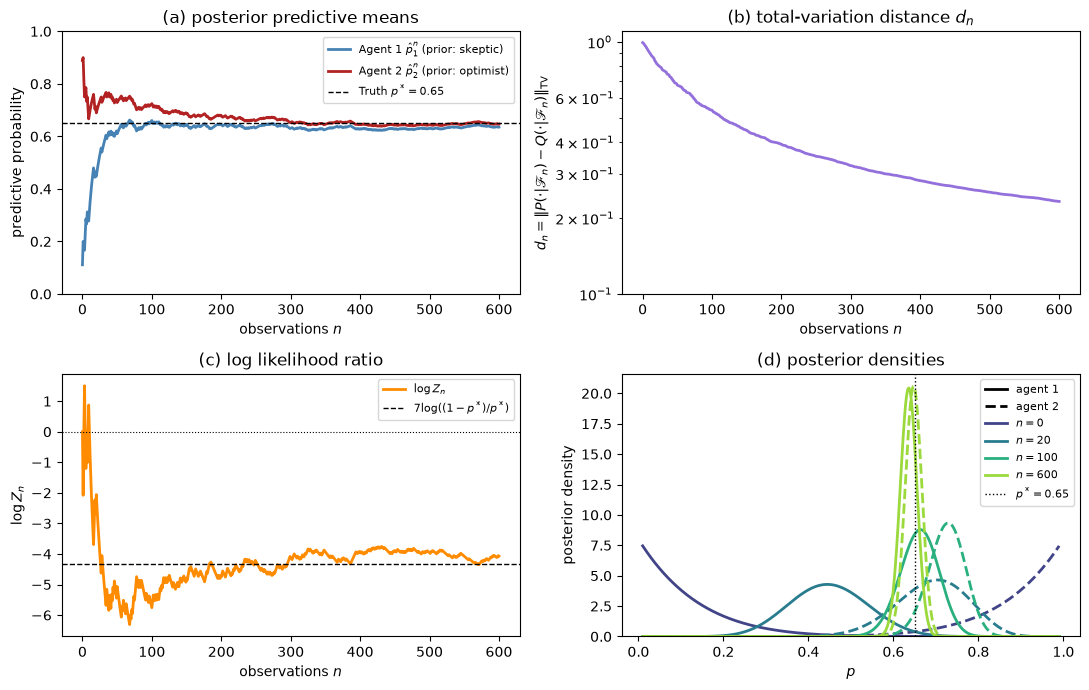
Fig. 34.1 Merging in the Beta–Bernoulli example. The four panels show posterior predictive means, the total-variation distance \(d_n\), the log likelihood ratio \(\log Z_n\), and posterior densities at selected horizons.#
k_n/n at n = 600: 0.643
d_n at n = 600: 0.233
log Z_n at n = 600: -4.07
7 log((1 - k_n/n) / (k_n/n)): -4.13
7 log((1 - p*) / p*): -4.33
The four panels show:
Panel (a): Starting from \(\hat{p}_1^0 \approx 0.11\) and \(\hat{p}_2^0 \approx 0.89\), both agents’ predictive probabilities converge to \(p^* = 0.65\).
Panel (b): The total-variation distance \(d_n\) falls from \(0.99\) to \(0.23\) at \(n = 600\).
Panel ©: The log likelihood ratio \(\log Z_n\) settles near \(7 \log((1-p^*)/p^*) = -4.33\), the closed-form limit at \(\bar p = p^*\). At \(n = 600\) the path has \(k_n/n = 0.643\), \(\log Z_n = -4.07\), and \(7 \log((1 - k_n/n)/(k_n/n)) = -4.13\).
Panel (d): The posterior Beta densities for the two agents start far apart (one near 0, one near 1) and progressively concentrate to the same distribution centred on the truth.
34.5.5. Almost-sure convergence across many paths#
To illustrate the almost-sure character of the theorem, we run many independent replications.
Each replication draws \(p\) from agent 1’s prior \(\pi_1 = \mathrm{Beta}(1, 8)\) and then draws \(x_1, x_2, \ldots\) IID Bernoulli\((p)\).
Each path is then a draw from \(P_1\).
With \(Q = P_1\) and \(P = P_2\), the theorem says that \(d_n \to 0\) on \(Q\)-almost every path.
N_paths = 80
n_steps = 2000

rng_p = np.random.default_rng(1234)
p_draws = rng_p.beta(a1, b1, N_paths)    # p drawn from agent 1's prior

tv_all   = np.empty((N_paths, n_steps + 1))
logZ_all = np.empty((N_paths, n_steps + 1))
steps    = np.arange(n_steps + 1)

for i in range(N_paths):
    s = run_simulation(p_draws[i], a1, b1, a2, b2, n_steps, seed=i)
    tv_all[i]   = s['tv_beta']
    logZ_all[i] = s['log_Z']

log_Z_limits = 7 * np.log((1 - p_draws) / p_draws)
norm_p = plt.Normalize(0, p_draws.max())
cmap = plt.cm.viridis

fig, axes = plt.subplots(1, 2, figsize=(11, 4))
ax_tv, ax_log = axes

for i in range(N_paths):
    col = cmap(norm_p(p_draws[i]))
    ax_tv.semilogy(steps, tv_all[i], color=col, lw=0.8, alpha=0.5)
    ax_log.plot(steps, logZ_all[i], color=col, lw=0.8, alpha=0.5)
ax_tv.semilogy(steps, tv_all.mean(axis=0),
               color='black', lw=2, label='mean across paths')
ax_tv.set_xlabel('observations $n$')
ax_tv.set_ylabel(r'$d_n$ (log scale)')
ax_tv.legend()

ax_log.scatter(np.full(N_paths, n_steps), log_Z_limits,
               c=p_draws, cmap=cmap, norm=norm_p, s=12, zorder=3,
               label=r'limit $7 \log((1-p)/p)$')
ax_log.axhline(0, color='gray', lw=0.8, ls=':')
ax_log.set_xlabel('observations $n$')
ax_log.set_ylabel(r'$\log Z_n$')
ax_log.legend()

fig.colorbar(plt.cm.ScalarMappable(norm=norm_p, cmap=cmap),
             ax=axes, label='$p$ drawn from $\\pi_1$')
plt.show()

for n in (500, n_steps):
    print(f"n = {n}: fraction of paths with d_n < 0.30 = "
          f"{np.mean(tv_all[:, n] < 0.30):.2f}, "
          f"mean d_n = {tv_all[:, n].mean():.3f}")
slow = np.argsort(tv_all[:, -1])[-5:]
print(f"p on the five slowest paths: {np.round(p_draws[slow], 4)}")
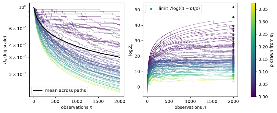
Fig. 34.2 Almost-sure merging across many sample paths drawn from \(P_1\). The left panel plots the total-variation distance and the right panel plots the log likelihood ratio \(\log Z_n\). Line colors record the value of \(p\) drawn on each path; dots mark the limits \(7 \log((1-p)/p)\).#
n = 500: fraction of paths with d_n < 0.30 = 0.14, mean d_n = 0.489
n = 2000: fraction of paths with d_n < 0.30 = 0.68, mean d_n = 0.299
p on the five slowest paths: [0.0036 0.0016 0.0035 0.0006 0.0016]
On every path \(d_{2000}\) is below \(d_0\), but on many paths \(d_n\) falls slowly.
At \(n = 500\), 14 percent of paths have \(d_n < 0.30\) and the mean of \(d_n\) is \(0.489\); at \(n = 2000\) the figures are 68 percent and \(0.299\).
The slowest paths have \(p\) below \(0.004\).
Agent 2’s prior density \(8p^7\) is tiny near \(p = 0\), so agent 2 needs many observations to move posterior mass there.
These finite-horizon numbers are consistent with the theorem, because almost-sure convergence is an asymptotic statement.
34.5.6. Is \(d_n\) a supermartingale?#
The proof of the theorem uses no monotonicity of \(\{d_n\}\).
In general, \(\{d_n\}\) is neither a \(P\)-supermartingale nor a \(Q\)-supermartingale.
A five-point example shows this.
Let \(\Omega = \{1, 2, 3, 4, 5\}\), let \(P\) be uniform, and let \(Z_\infty = dQ/dP = (0, 1, 1, 1, 2)\).
A first observation reveals whether \(\omega \in \{1, 2\}\) or \(\omega \in \{3, 4, 5\}\), and a second observation reveals \(\omega\).
P_pts = np.full(5, 0.2)
Q_pts = np.array([0, 1, 1, 1, 2]) * P_pts
blocks = [[0, 1], [2, 3, 4]]      # cells revealed by the first observation

d_0 = 0.5 * np.abs(P_pts - Q_pts).sum()
E_Q_d1 = E_P_d1 = 0.0
for b in blocks:
    P_b, Q_b = P_pts[b].sum(), Q_pts[b].sum()
    d_1 = 0.5 * np.abs(P_pts[b] / P_b - Q_pts[b] / Q_b).sum()
    E_Q_d1 += Q_b * d_1
    E_P_d1 += P_b * d_1

print(f"d_0 = {d_0:.3f}, E_Q[d_1] = {E_Q_d1:.3f}, E_P[d_1] = {E_P_d1:.3f}")
d_0 = 0.200, E_Q[d_1] = 0.233, E_P[d_1] = 0.300
Here \(d_0 = 0.200\), \(\mathbb{E}_Q[d_1] = 0.233\), and \(\mathbb{E}_P[d_1] = 0.300\).
The first observation raises the expected distance under both measures.
The second observation reveals \(\omega\), so \(d_2 = 0\).
The identity \(2\,\mathbb{E}_Q[d_n] = \mathbb{E}_P[|Z_\infty - Z_n|]\) locates the source of the failure: the \(L^1\) distance between \(Z_\infty\) and its conditional expectation given \(\mathscr{F}_n\) need not decrease with \(n\).
When \(\mathbb{E}_P[Z_\infty^2] < \infty\), the \(L^2\) distance does decrease, because \(\mathbb{E}_P[(Z_\infty - Z_n)^2] = \mathbb{E}_P[Z_\infty^2] - \mathbb{E}_P[Z_n^2]\) and \(\mathbb{E}_P[Z_n^2]\) is nondecreasing in \(n\).
In the Beta–Bernoulli model with the priors above, the inequality \(\mathbb{E}[d_{n+1} \,|\, \mathscr{F}_n] \leq d_n\) holds at every state we check.
The next cell computes \(\mathbb{E}_Q[d_{n+1} \,|\, \mathscr{F}_n] - d_n\) and \(\mathbb{E}_P[d_{n+1} \,|\, \mathscr{F}_n] - d_n\) exactly at every state \((n, k_n)\) with \(n < 400\), using each agent’s one-step predictive probability.
def conditional_increments(n, a1, b1, a2, b2):
    """
    E_Q[d_{n+1} | n, k] - d_n and E_P[d_{n+1} | n, k] - d_n
    for k = 0, ..., n, with Q = P_1 and P = P_2.
    """
    k = np.arange(n + 1)
    d_now  = tv_distance_beta(a1 + k, b1 + n - k, a2 + k, b2 + n - k)
    d_head = tv_distance_beta(a1 + k + 1, b1 + n - k,
                              a2 + k + 1, b2 + n - k)
    d_tail = tv_distance_beta(a1 + k, b1 + n - k + 1,
                              a2 + k, b2 + n - k + 1)
    q1 = (a1 + k) / (a1 + b1 + n)        # agent 1's predictive probability
    q2 = (a2 + k) / (a2 + b2 + n)        # agent 2's predictive probability
    inc_Q = q1 * d_head + (1 - q1) * d_tail - d_now
    inc_P = q2 * d_head + (1 - q2) * d_tail - d_now
    return inc_Q, inc_P

n_check = 400
max_inc_Q = np.empty(n_check)
max_inc_P = np.empty(n_check)
for n in range(n_check):
    inc_Q, inc_P = conditional_increments(n, a1, b1, a2, b2)
    max_inc_Q[n], max_inc_P[n] = inc_Q.max(), inc_P.max()

fig, axes = plt.subplots(1, 2, figsize=(11, 4))

ax = axes[0]
for n, col in zip([20, 100, 399], ['steelblue', 'darkorange', 'firebrick']):
    inc_Q, _ = conditional_increments(n, a1, b1, a2, b2)
    ax.plot(np.arange(n + 1) / n, inc_Q, color=col, lw=2, label=f'$n={n}$')
ax.axhline(0, color='black', lw=0.8, ls='--')
ax.set_xlabel('$k_n / n$')
ax.set_ylabel(r'$\mathbb{E}_Q[d_{n+1} | \mathscr{F}_n] - d_n$')
ax.legend(fontsize=8)

ax = axes[1]
ax.plot(max_inc_Q, color='purple', lw=2, label='under $Q = P_1$')
ax.plot(max_inc_P, color='gray', lw=2, ls='--', label='under $P = P_2$')
ax.axhline(0, color='black', lw=0.8, ls=':')
ax.set_xlabel('observations $n$')
ax.set_ylabel(r'largest increment over $k_n$')
ax.legend(fontsize=8)

plt.tight_layout()
plt.show()

print(f"Largest increment under Q over all states: {max_inc_Q.max():.2e}")
print(f"Largest increment under P over all states: {max_inc_P.max():.2e}")
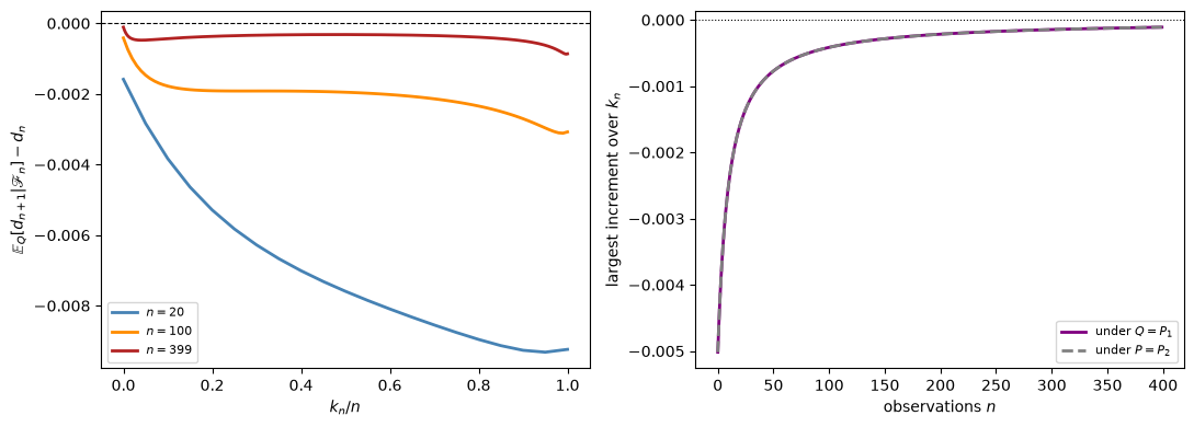
Fig. 34.3 Exact one-step conditional increments of \(d_n\) in the Beta–Bernoulli model. The left panel plots \(\mathbb{E}_Q[d_{n+1} | \mathscr{F}_n] - d_n\) against \(k_n/n\) for selected \(n\). The right panel plots the largest increment over all \(k_n\) at each \(n\).#
Largest increment under Q over all states: -1.10e-04
Largest increment under P over all states: -1.10e-04
Every increment is negative, so in this model \(\{d_n\}\) behaves as a supermartingale under both \(P_1\) and \(P_2\) over the states we check.
The two curves in the right panel coincide because \(\pi_2(p) = \pi_1(1-p)\): exchanging heads and tails exchanges the two agents.
The supermartingale property is specific to the model; the five-point example shows that it fails in general.
34.6. Failure of merging: mutual singularity#
What happens when the hypothesis \(Q \ll P\) fails?
The singular case is the cleanest counterexample.
34.6.1. Point-mass priors#
Suppose both agents hold degenerate (point-mass) priors:
Agent P: certain that \(p = p_P = 0.30\).
Agent Q: certain that \(p = p_Q = 0.75\).
Since \(P\) charges only sequences whose empirical frequency converges to \(0.30\), and \(Q\) charges only sequences whose empirical frequency converges to \(0.75\), the two measures are mutually singular: \(P \perp Q\).
The conditional distributions do not update, because both agents are already certain of their model.
For the theorem’s object, namely the conditional law of the entire future path,
This equality holds because the infinite-product Bernoulli measures with distinct success probabilities are singular.
If we look only one step ahead, the predictive distance is \(|p_P - p_Q| = 0.45\).
That is smaller than one, but it is not the quantity that appears in Blackwell–Dubins.
p_P = 0.30
p_Q = 0.75
n_steps = 500

tv_singular_full = np.ones(n_steps + 1)
tv_singular_1step = np.full(n_steps + 1, np.abs(p_P - p_Q))

sim_abs_cont = run_simulation(
    p_Q, 1.0, 8.0, 8.0, 1.0, n_steps, seed=1
)

fig, ax = plt.subplots(figsize=(8, 4))
ax.plot(np.arange(n_steps + 1), tv_singular_full,
        color='firebrick', lw=2,
        label=r'singular: full-path $d_n = 1$')
ax.plot(np.arange(n_steps + 1), tv_singular_1step,
        color='gray', lw=2, ls=':',
        label=r'one-step gap $= |p_P - p_Q|$')
ax.plot(np.arange(n_steps + 1),
        sim_abs_cont['tv_beta'],
        color='steelblue', lw=2,
        label=(r'$\mathrm{Beta}(1,8)$ vs'
               r' $\mathrm{Beta}(8,1)$'))
ax.set_xlabel('observations $n$')
ax.set_ylabel(r'$d_n$')
ax.legend(fontsize=8)
ax.set_ylim(0, 1.05)

plt.tight_layout()
plt.show()
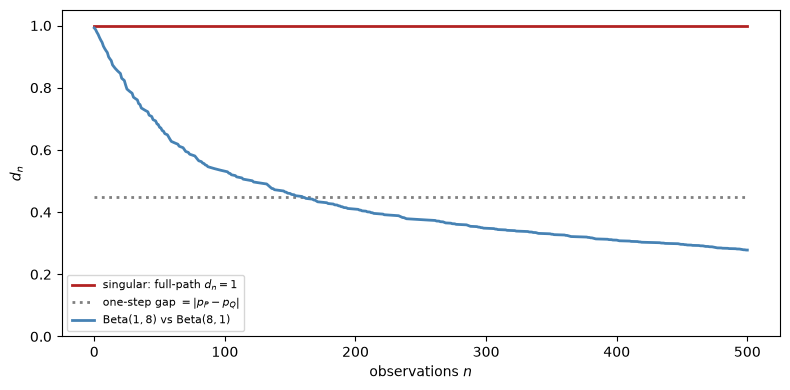
Fig. 34.4 Failure of merging under singular priors. The full future-path distance stays at one, while the one-step predictive gap stays at \(|p_P - p_Q|\).#
The contrast is sharp.
With mutually absolutely continuous priors, \(d_n\) decays to zero on a path generated by a coin with \(p = 0.75\).
With singular point-mass priors, the full future-path distance stays at one forever.
More data does not reconcile the agents, because each rules out paths the other assigns positive probability.
34.7. Kakutani’s theorem: when does merging hold?#
A natural question is: for which product measures does the Blackwell–Dubins hypothesis \(Q \ll P\) hold?
For infinite product measures, the answer is given by a classical result of Kakutani [1948].
34.7.1. Hellinger affinities#
In this section \(P^{(m)}\) and \(Q^{(m)}\) denote probability measures on the signal space \((S, \mathscr{S})\), the factors of product measures.
The notation \(P_n\) and \(Q_n\) keeps its earlier meaning: restrictions of \(P\) and \(Q\) to \(\mathscr{F}_n\).
Definition 34.3 (Hellinger Affinity)
For probability measures \(P^{(m)}\) and \(Q^{(m)}\) on \((S, \mathscr{S})\) with common dominating measure \(\lambda\), the Hellinger affinity is
\(\rho_m = 1\) if and only if \(P^{(m)} = Q^{(m)}\); \(\rho_m = 0\) if and only if \(P^{(m)} \perp Q^{(m)}\).
The Hellinger affinity is the Bhattacharyya coefficient, the Chernoff coefficient at \(\phi = 1/2\) in Statistical Divergence Measures.
For two specific one-dimensional families:
Gaussian: \(P^{(m)} = \mathcal{N}(0, 1)\) vs \(Q^{(m)} = \mathcal{N}(\mu_m,1)\):
Bernoulli: \(P^{(m)} = \mathrm{Bernoulli}(p)\) vs \(Q^{(m)} = \mathrm{Bernoulli}(q)\):
34.7.2. Kakutani’s dichotomy#
Theorem 34.2 (Kakutani (1948))
Let \(P = \bigotimes_{m=1}^\infty P^{(m)}\) and \(Q = \bigotimes_{m=1}^\infty Q^{(m)}\) be infinite product measures whose factors are pairwise equivalent: \(P^{(m)} \sim Q^{(m)}\) for every \(m\).
Then either \(P \sim Q\) or \(P \perp Q\); there is no intermediate case.
Specifically,
If \(\prod_{m=1}^\infty \rho_m = 0\), then \(P \perp Q\).
Proof idea. A standard proof studies the likelihood-ratio martingale \(Z_N = \prod_{m=1}^N (dQ^{(m)}/dP^{(m)})\) together with the identity \(\mathbb{E}_P[\sqrt{Z_N}] = \prod_{m=1}^N \rho_m\).
If the product is positive, \(\{\sqrt{Z_N}\}\) is Cauchy in \(L^2(P)\), so \(Z_N\) converges in \(L^1(P)\) and \(Q \ll P\); the same argument with \(P\) and \(Q\) exchanged gives \(P \ll Q\).
If the product is zero, Fatou’s lemma gives \(\mathbb{E}_P[\sqrt{Z_\infty}] = 0\), so \(Z_\infty = 0\) \(P\)-a.s. and \(P \perp Q\).
\(\square\)
34.7.3. Implication for merging#
For IID-type sequences, Kakutani’s theorem gives the following picture:
Scenario |
\(\sum_m (1-\rho_m)\) |
Conclusion |
Merging? |
|---|---|---|---|
\(P^{(m)} = Q^{(m)}\) for all \(m\) |
\(0\) |
\(P = Q\) |
Trivially yes |
\(P^{(m)} \ne Q^{(m)}\) with \(\sum_m (1-\rho_m) < \infty\) |
Finite |
\(P \sim Q\) |
Yes; Blackwell–Dubins applies |
\(P^{(m)} = f \ne g = Q^{(m)}\) for all \(m\) |
\(\infty\) |
\(P \perp Q\) |
No |
The IID case with different fixed marginals is the standard no-merging example.
If two agents assign permanently different distributions to each observation, they end up in disjoint probability worlds.
Likelihood Ratio Processes shows the likelihood ratio process converging to zero when nature permanently draws from one of two fixed densities.
For product measures, the conditional distribution of the future given \(\mathscr{F}_n\) does not depend on the past.
So \(d_n = \bigl\|\bigotimes_{m>n} P^{(m)} - \bigotimes_{m>n} Q^{(m)}\bigr\|_{\mathrm{TV}}\) is deterministic.
Each \(\rho_m\) is positive because the factors are equivalent, so dropping finitely many factors does not change whether \(\prod_m \rho_m\) is positive.
When \(P \perp Q\), the products over \(m > n\) are singular, and \(d_n = 1\) for every \(n\).
When \(P \sim Q\), \(d_n \to 0\) by Blackwell–Dubins.
Exercise 34.3 computes \(d_n\) exactly for Gaussian products.
34.7.4. A Gaussian product-measure example#
We illustrate Kakutani’s dichotomy with Gaussian product measures.
Take \(P = \mathcal{N}(0,1)^{\otimes\mathbb{N}}\) as the reference measure and \(Q = \bigotimes_m \mathcal{N}(\mu_m,1)\) as the alternative.
Then \(\log Z_N = \sum_{m=1}^N (\mu_m x_m - \mu_m^2/2)\), and the code below draws \(x_m\) from \(\mathcal{N}(0, 1)\), that is, under \(P\).
Three choices of \(\mu_m\):
\(\mu_m = \mu > 0\) constant (\(\sum (1-\rho_m) = \infty\)) \(\Rightarrow P \perp Q\).
\(\mu_m = c/\!\sqrt{m}\) (\(\sum (1-\rho_m) \approx \sum c^2/(8m) = \infty\)) \(\Rightarrow P \perp Q\).
\(\mu_m = c/m\) (\(\sum (1-\rho_m) \approx \sum c^2/(8m^2) < \infty\)) \(\Rightarrow P \sim Q\).
N_max  = 2000
ms     = np.arange(1, N_max + 1)
c      = 2.0
N_plot = 400
rng    = np.random.default_rng(0)

cases = [
    (r'$\mu_m = c$ (constant)', np.full(N_max, c)),
    (r'$\mu_m = c/\sqrt{m}$', c / np.sqrt(ms)),
    (r'$\mu_m = c/m$', c / ms),
]
With constant drift, \(\log Z_N\) drifts to \(-\infty\) under \(P\), so \(Z_N \to 0\) \(P\)-a.s. and \(P \perp Q\).
label, μ_seq = cases[0]
x = rng.standard_normal(N_plot)
log_Z_inc = μ_seq[:N_plot] * x - μ_seq[:N_plot]**2 / 2
log_Z = np.concatenate([[0], np.cumsum(log_Z_inc)])

fig, ax = plt.subplots(figsize=(8, 3))
ax.plot(np.arange(N_plot + 1), log_Z,
        color='darkorange', lw=2, label=label)
ax.axhline(0, color='black', lw=0.8, ls=':')
ax.set_xlabel('horizon $N$')
ax.set_ylabel(r'$\log Z_N$ under $P$')
ax.legend(fontsize=8)
plt.tight_layout()
plt.show()
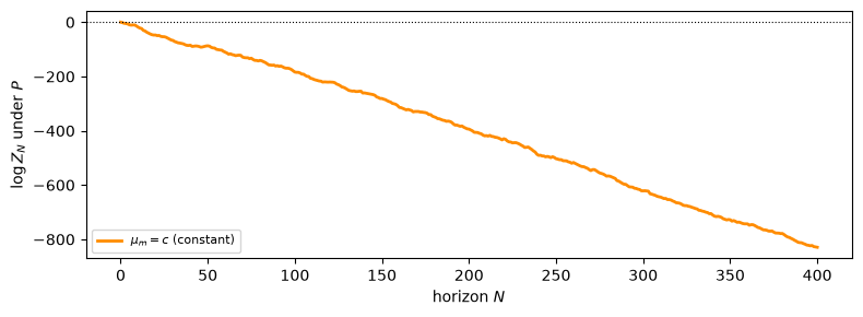
Fig. 34.5 Constant drift \(\mu_m = c\): the likelihood ratio collapses (\(P \perp Q\)).#
The \(\mu_m = c/\sqrt{m}\) case shows the same qualitative picture: despite the drift vanishing, it does so too slowly.
label, μ_seq = cases[1]
x = rng.standard_normal(N_plot)
log_Z_inc = μ_seq[:N_plot] * x - μ_seq[:N_plot]**2 / 2
log_Z = np.concatenate([[0], np.cumsum(log_Z_inc)])

fig, ax = plt.subplots(figsize=(8, 3))
ax.plot(np.arange(N_plot + 1), log_Z,
        color='purple', lw=2, label=label)
ax.axhline(0, color='black', lw=0.8, ls=':')
ax.set_xlabel('horizon $N$')
ax.set_ylabel(r'$\log Z_N$ under $P$')
ax.legend(fontsize=8)
plt.tight_layout()
plt.show()
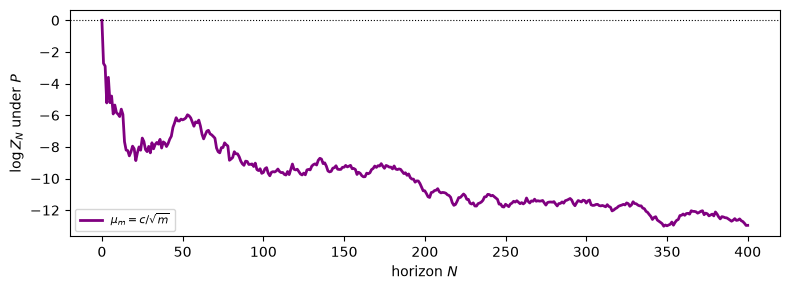
Fig. 34.6 Drift \(\mu_m = c/\sqrt{m}\): still singular (\(P \perp Q\)).#
Only with \(\mu_m = c/m\) does \(\sum (1-\rho_m) < \infty\) hold, so the likelihood ratio remains nondegenerate and \(P \sim Q\).
Blackwell–Dubins applies only in this case.
label, μ_seq = cases[2]
x = rng.standard_normal(N_plot)
log_Z_inc = μ_seq[:N_plot] * x - μ_seq[:N_plot]**2 / 2
log_Z = np.concatenate([[0], np.cumsum(log_Z_inc)])

fig, ax = plt.subplots(figsize=(8, 3))
ax.plot(np.arange(N_plot + 1), log_Z,
        color='steelblue', lw=2, label=label)
ax.axhline(0, color='black', lw=0.8, ls=':')
ax.set_xlabel('horizon $N$')
ax.set_ylabel(r'$\log Z_N$ under $P$')
ax.legend(fontsize=8)
plt.tight_layout()
plt.show()
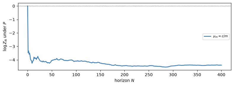
Fig. 34.7 Drift \(\mu_m = c/m\): the likelihood ratio stabilises (\(P \sim Q\)).#
34.8. Extension to continuous time#
The same logic extends to continuous time.
34.8.1. Girsanov’s theorem and the likelihood-ratio process#
On the canonical Wiener space with \(P\) the Wiener measure (standard Brownian motion \(W\)), suppose agent \(Q\) believes the process has an additional drift \(\theta = \{\theta_s\}_{s \geq 0}\):
where \(\widetilde{W}\) is a \(Q\)-Brownian motion.
The Girsanov–Cameron–Martin theorem [Girsanov, 1960] gives the likelihood-ratio process \(Z_t = dQ_t/dP_t\) as the stochastic exponential
\(Z_t\) is always a non-negative \(P\)-local martingale; it is a true martingale if and only if \(\mathbb{E}_P[Z_t] = 1\) for all \(t\).
Novikov’s condition [Novikov, 1972], \(\mathbb{E}_P\!\left[\exp\!\left(\tfrac{1}{2}\int_0^T \theta_s^2\,ds\right)\right] < \infty\) for all \(T\), is sufficient.
34.8.2. The dichotomy at infinity#
A key subtlety on \([0,+\infty)\) is that local absolute continuity does not imply global absolute continuity on \(\mathscr{F}_\infty\).
Remark 34.3 (Infinite-Horizon Subtlety)
Suppose \(Z_t\) is a true \(P\)-martingale for every finite horizon and let \(Z_t \to Z_\infty\) \(P\)-a.s.
If \(\{Z_t\}\) is uniformly integrable on \([0,\infty)\), then \(Q \ll P\) on \(\mathscr{F}_\infty\) with \(dQ/dP = Z_\infty\).
That is the hypothesis of Blackwell–Dubins, so merging holds \(Q\)-a.s.
If in addition \(Z_\infty > 0\) \(P\)-a.s., then \(P \ll Q\) as well, and merging holds \(P\)-a.s.
Merging \(P\)-a.s. requires only \(P \ll Q\), because \(d_t\) is symmetric in \(P\) and \(Q\) and the theorem applies with their roles exchanged.
If uniform integrability fails, then global absolute continuity on \(\mathscr{F}_\infty\) can fail.
In many standard examples, including a non-zero constant drift, the measures are in fact singular on \(\mathscr{F}_\infty\).
For a deterministic drift \(\theta\), the energy condition
separates the two cases.
If it holds, \(\mathbb{E}_P[Z_t^2] = \exp\!\left(\int_0^t \theta_s^2\, ds\right)\) is bounded in \(t\), \(\{Z_t\}\) is uniformly integrable, \(Z_\infty > 0\), and \(P \sim Q\) on \(\mathscr{F}_\infty\).
If it fails, \(\log Z_t \to -\infty\) \(P\)-a.s. and \(P \perp Q\) on \(\mathscr{F}_\infty\).
Informally, \(\int_0^\infty \theta_s^2\,ds\) measures the total amount of information separating the two measures over the infinite horizon.
Under the energy condition, Blackwell–Dubins applies and merging holds under both measures.
When \(\theta\) is a non-zero constant, the condition fails, the measures are singular on \(\mathscr{F}_\infty\), and merging does not occur.
Survival and Long-Run Dynamics under Recursive Preferences studies agents whose beliefs differ from the truth by a constant drift of this kind.
When \(\theta\) depends on the path of \(W\), \(\int_0^\infty \theta_s^2\,ds\) is a random variable.
In that case \(P \sim Q\) on \(\mathscr{F}_\infty\) if and only if \(\int_0^\infty \theta_s^2\,ds < \infty\) both \(P\)-a.s. and \(Q\)-a.s.
Under \(P\), \(\log Z_t = \int_0^t \theta_s\,dW_s - \tfrac{1}{2}\int_0^t \theta_s^2\,ds\) tends to \(-\infty\) on the event \(\{\int_0^\infty \theta_s^2\,ds = \infty\}\).
Under \(Q\), \(\log Z_t = \int_0^t \theta_s\,d\widetilde{W}_s + \tfrac{1}{2}\int_0^t \theta_s^2\,ds\) tends to \(+\infty\) on the same event.
On the complementary event, \(\log Z_t\) converges to a finite limit under both measures.
Since \(Q \ll P\) on \(\mathscr{F}_\infty\) if and only if \(Z_\infty < \infty\) \(Q\)-a.s., and \(P \ll Q\) if and only if \(Z_\infty > 0\) \(P\)-a.s., the claim follows.
Whenever \(Q \ll P\) on \(\mathscr{F}_\infty\) is established, the discrete-time proof carries over.
The conditional distance satisfies \(d_t = \mathbb{E}_P[|Z_\infty - Z_t| \,|\, \mathscr{F}_t]/(2 Z_t)\), \(Z_t \to Z_\infty > 0\) \(Q\)-a.s., and the truncation argument in Step 3 sends the numerator to zero.
The identity \(\mathbb{E}_Q[d_t] = \tfrac{1}{2}\mathbb{E}_P[|Z_t - Z_\infty|]\) also carries over.
34.9. Applications#
34.9.1. Bayesian learning#
The most direct application is Bayesian inference.
Suppose data \((x_1, x_2, \ldots)\) are drawn from the true measure \(Q^*\).
An agent holds a prior \(\pi\) over a family \(\{Q_\theta : \theta \in \Theta\}\), inducing a marginal \(P = \int Q_\theta\,\pi(d\theta)\).
If \(Q^* \ll P\) (i.e., the agent’s marginal model dominates the truth), then Blackwell–Dubins gives
This is a strong form of Bayesian consistency: the agent’s predictions merge with the truth under the true measure.
A prior assigning positive mass to a neighbourhood of the true parameter typically guarantees local absolute continuity \(Q^*_n \ll P_n\) for every finite horizon \(n\), but not the global condition \(Q^* \ll P\) on \(\mathscr{F}_\infty\) that Blackwell–Dubins requires.
For example, in the Beta–Bernoulli model with a non-atomic prior \(\pi\), the mixture \(P = \int \mathrm{Bernoulli}(p)^{\infty}\,\pi(dp)\) satisfies \(Q^*_n \ll P_n\) for every \(n\), yet \(Q^* \not\ll P\) globally because the set \(\{\lim k_n/n = p^*\}\) has \(Q^*\)-measure one but \(P\)-measure zero (different Bernoulli product measures are mutually singular).
In an identifiable IID family, the measures \(Q_\theta\) for distinct \(\theta\) are mutually singular, so \(Q_{\theta^*} \ll P\) if and only if \(\pi(\{\theta^*\}) > 0\).
Global absolute continuity therefore holds when \(\pi\) has an atom at \(\theta^*\), for example when \(\Theta\) is finite.
Likelihood Ratio Processes and Bayesian Learning studies an agent whose prior puts positive probability on each of two models, one of which is true; there \(Q^* \ll P\).
With a non-atomic prior, the agent’s forecasts of the entire future never merge with the truth.
In the Beta–Bernoulli model, the argument that gave the closed form for \(d_n\) gives \(\|P_i(\,\cdot\,|\,\mathscr{F}_n) - P_{p^*}(\,\cdot\,|\,\mathscr{F}_n)\|_{\mathrm{TV}} = 1\) for every \(n\), because agent \(i\)’s posterior has no atom at \(p^*\).
Each agent’s one-step-ahead forecast still converges to \(p^*\), and the two agents’ forecasts merge with each other.
Doob’s consistency theorem [Doob, 1949] states that the posterior concentrates at the true \(\theta\) for \(\pi\)-almost every \(\theta\).
Diaconis and Freedman [1986] study consistency at a fixed parameter value, where Doob’s theorem is silent.
They show that in infinite-dimensional models the exceptional \(\pi\)-null set can matter: in a location problem with a Dirichlet-process prior on the error distribution, the posterior can be inconsistent at parameter values in the support of the prior.
In Incorrect Models, nature draws IID from a mixture \(h\) of densities \(f\) and \(g\), while the agent believes that nature drew once and for all from \(f\) or from \(g\).
There \(P \perp Q^*\), the agent’s forecasts stay wrong, and the agent’s posterior concentrates on the model closer to \(h\) in Kullback–Leibler divergence.
34.9.2. Rational expectations and heterogeneous priors#
In macroeconomics, rational-expectations models typically impose a common prior.
Blackwell–Dubins gives a dynamic justification for weaker initial agreement.
If two agents start with equivalent priors and observe the same history, their conditional forecasts eventually agree on every event.
Aumann [1976]’s agreement theorem complements this result.
Aumann’s agents share a common prior and see different private information; if their posterior probabilities of an event are common knowledge, the posteriors are equal.
Blackwell and Dubins’s agents hold different priors and see the same information.
When merging fails, disagreement persists and has economic consequences.
Heterogeneous Beliefs and Financial Markets studies how wealth moves between agents with different beliefs, including an agent whose prior rules out the true model.
Survival and Long-Run Dynamics under Recursive Preferences studies which agents survive when beliefs differ permanently.
34.9.3. Ergodic Markov chains#
For a Markov chain with transition kernel \(\Pi\) and two initial distributions \(\mu\) and \(\nu\), the \(n\)-step distributions are \(\mu\Pi^n\) and \(\nu\Pi^n\).
If \(\Pi\) is ergodic with unique stationary distribution \(\pi\), both converge to \(\pi\), so
This convergence does not require absolute continuity: \(\mu\) and \(\nu\) can be point masses at different states.
It concerns a different object from Blackwell–Dubins.
The measures \(\mu\Pi^n\) and \(\nu\Pi^n\) are unconditional distributions of the state at date \(n\), and their convergence says that an ergodic chain forgets its initial condition.
Blackwell–Dubins concerns conditional distributions of the entire future given a common observed history.
Two agents who agree on \(\Pi\) and observe the current state make identical conditional forecasts of the future, whether or not \(\Pi\) is ergodic.
34.10. The rate of merging#
Blackwell–Dubins is qualitative.
It tells us that \(d_n \to 0\), but not how fast.
The identity
shows that the rate of merging in \(Q\)-mean is governed by the \(L^1(P)\) convergence rate of the likelihood-ratio martingale.
In regular parametric examples, one often sees \(n^{-1/2}\)-type behavior.
In the Beta–Bernoulli model, the normal approximation derived earlier gives \(d_n \approx 7/\sqrt{2 \pi n\, \hat p_n (1 - \hat p_n)}\).
Under a fixed coin \(P_{p^*}\), \(\hat p_n \to p^*\), so \(\mathbb{E}_{P_{p^*}}[d_n] \approx C(p^*)/\sqrt{n}\) with \(C(p^*) = 7/\sqrt{2\pi p^*(1-p^*)}\) and \(C(0.65) = 5.85\).
Under \(Q = P_1\), the coin \(p\) is drawn from \(\pi_1\), and averaging over \(p\) gives \(\mathbb{E}_Q[d_n] \approx C_Q/\sqrt{n}\) with
The next cell computes both expectations exactly by summing \(d_n\) over the number of successes \(k_n\), which is binomial under \(P_{p^*}\) and beta-binomial under \(Q = P_1\).
def expected_d(n):
    """Exact E_{P_{p*}}[d_n] and E_Q[d_n], with Q = P_1."""
    k = np.arange(n + 1)
    d = tv_distance_beta(a1 + k, b1 + n - k, a2 + k, b2 + n - k)
    return binom.pmf(k, n, p_true) @ d, betabinom.pmf(k, n, a1, b1) @ d

n_grid = np.unique(np.logspace(0, 4, 60).astype(int))
mean_fixed, mean_Q = np.array([expected_d(n) for n in n_grid]).T

C_fixed = 7 / np.sqrt(2 * np.pi * p_true * (1 - p_true))
C_Q = 7 / np.sqrt(2 * np.pi) * beta_fn(0.5, 7.5) / beta_fn(a1, b1)

fig, ax = plt.subplots(figsize=(8, 4))
ax.loglog(n_grid, mean_fixed, color='steelblue', lw=2,
          label=r'$\mathbb{E}_{P_{0.65}}[d_n]$')
ax.loglog(n_grid, C_fixed / np.sqrt(n_grid), color='steelblue',
          lw=1.5, ls='--', label=rf'${C_fixed:.2f}/\sqrt{{n}}$')
ax.loglog(n_grid, mean_Q, color='firebrick', lw=2,
          label=r'$\mathbb{E}_Q[d_n]$, $Q = P_1$')
ax.loglog(n_grid, C_Q / np.sqrt(n_grid), color='firebrick',
          lw=1.5, ls='--', label=rf'${C_Q:.1f}/\sqrt{{n}}$')
ax.set_ylim(1e-2, 1.5)
ax.set_xlabel('sample size $n$')
ax.set_ylabel('mean of $d_n$')
ax.legend()
plt.tight_layout()
plt.show()

for n in (100, 500, 1000, 10_000):
    e_fixed, e_Q = expected_d(n)
    δ, s = 7 / (n + 9), np.sqrt(p_true * (1 - p_true) / n)
    print(f"n = {n:>6}: E_P0.65[d_n] = {e_fixed:.3f}, "
          f"normal approx = {2 * norm.cdf(δ / (2 * s)) - 1:.3f}, "
          f"C/sqrt(n) = {C_fixed / np.sqrt(n):.3f} | "
          f"E_Q[d_n] / (C_Q/sqrt(n)) = {e_Q / (C_Q / np.sqrt(n)):.2f}")

late = n_grid >= 1000
for name, m in (("P_0.65", mean_fixed), ("Q", mean_Q)):
    slope = np.polyfit(np.log(n_grid[late]), np.log(m[late]), 1)[0]
    print(f"log-log slope under {name}, 1000 <= n <= 10^4: {slope:.2f}")
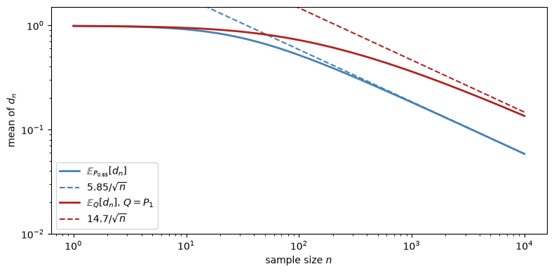
Fig. 34.8 Exact means of \(d_n\) in the Beta–Bernoulli model under a fixed coin \(P_{0.65}\) and under \(Q = P_1\). Dashed lines are the normal approximations \(C/\sqrt{n}\).#
n =    100: E_P0.65[d_n] = 0.519, normal approx = 0.499, C/sqrt(n) = 0.585 | E_Q[d_n] / (C_Q/sqrt(n)) = 0.49
n =    500: E_P0.65[d_n] = 0.255, normal approx = 0.253, C/sqrt(n) = 0.262 | E_Q[d_n] / (C_Q/sqrt(n)) = 0.70
n =   1000: E_P0.65[d_n] = 0.183, normal approx = 0.182, C/sqrt(n) = 0.185 | E_Q[d_n] / (C_Q/sqrt(n)) = 0.78
n =  10000: E_P0.65[d_n] = 0.058, normal approx = 0.058, C/sqrt(n) = 0.059 | E_Q[d_n] / (C_Q/sqrt(n)) = 0.92
log-log slope under P_0.65, 1000 <= n <= 10^4: -0.50
log-log slope under Q, 1000 <= n <= 10^4: -0.43
Under \(P_{0.65}\), the exact mean approaches \(5.85/\sqrt{n}\) from below.
At \(n = 500\), the exact mean is \(0.255\), the normal approximation \(2\Phi(\delta_n/(2 s_n)) - 1\) at \(\hat p_n = 0.65\) is \(0.253\), and \(5.85/\sqrt{n}\) is \(0.262\).
The fitted log-log slope over \(1000 \leq n \leq 10^4\) is \(-0.50\).
Under \(Q\), the approach to \(14.7/\sqrt{n}\) is slow.
The ratio of \(\mathbb{E}_Q[d_n]\) to \(14.7/\sqrt{n}\) is \(0.70\) at \(n = 500\) and \(0.92\) at \(n = 10^4\), and the fitted slope over \(1000 \leq n \leq 10^4\) is \(-0.43\).
The prior \(\pi_1\) puts much of its mass near \(p = 0\), where the normal approximation needs \(n p\) to be large.
34.11. Summary and extensions#
The logical flow underlying the Blackwell–Dubins theorem is:
Takeaways:
One-sided absolute continuity \(Q \ll P\) gives merging \(Q\)-almost surely. For merging under both measures, one needs mutual absolute continuity \(P \sim Q\).
The likelihood-ratio martingale \(Z_n = \mathbb{E}_P[Z|\mathscr{F}_n]\) drives the result: in \(d_n = \mathbb{E}_P[|Z - Z_n| \,|\, \mathscr{F}_n]/(2 Z_n)\), the numerator converges to zero and \(Z_n\) converges to \(Z > 0\), \(Q\)-a.s.
More data can only increase the ability to distinguish two hypotheses: \(\|P_n - Q_n\|_{\mathrm{TV}}\) on \(\mathscr{F}_n\) is nondecreasing in \(n\). The conditional distance \(d_n\) need not decrease, even in expectation. It converges to zero when \(Q \ll P\).
For infinite product measures, Kakutani’s theorem gives a sharp equivalence-versus-singularity dichotomy: either \(P \sim Q\) (when \(\sum_m (1 - \rho_m) < \infty\)) or \(P \perp Q\) (when the sum diverges), with no intermediate case.
When \(P \sim Q\), Blackwell–Dubins applies and merging occurs under both measures; when \(P \perp Q\) and \(P_n \sim Q_n\) for every \(n\), \(d_n = 1\) for every \(n\) and disagreement persists forever.
34.11.1. Applications in economics#
Some influential applications and extensions are:
[Kalai and Lehrer, 1993]: repeated-game learning drives play toward Nash behavior when priors are absolutely continuous with respect to the truth.
[Kalai and Lehrer, 1993]: subjective and objective equilibria coincide asymptotically under the same condition.
[Kalai and Lehrer, 1994]: weak and strong notions of merging are introduced for environments where full total-variation convergence is too strong.
[Kalai et al., 1999]: merging is linked to calibrated forecasting.
[Jackson et al., 1999]: de Finetti-style representations are connected to Bayesian learning and posterior convergence.
[Jackson and Kalai, 1999]: social learning erodes reputational effects that rely on persistent disagreement across cohorts.
[Sandroni, 1998]: near-absolute-continuity conditions are shown to suffice for Nash-type convergence in repeated games.
[Miller and Sanchirico, 1999]: gives an alternative proof and an economic interpretation of persistent disagreement in terms of mutually favorable bets.
[Lehrer and Smorodinsky, 1996]: studies broader compatibility notions beyond Blackwell–Dubins absolute continuity.
[Lehrer and Smorodinsky, 1996]: surveys merging and learning in repeated strategic environments.
[Nyarko, 1994]: relates Bayesian learning under absolute continuity to convergence toward correlated equilibrium.
[Pomatto et al., 2014]: extends the theorem to finitely additive probabilities and connects merging to test manipulability.
[Acemoglu et al., 2016]: shows how disagreement can persist when agents are uncertain about the signal structure itself.
34.12. Exercises#
Exercise 34.2
Let agent 1’s prior be \(\pi_1 = \mathrm{Unif}(0, \tfrac12)\) and agent 2’s prior be \(\pi_2 = \mathrm{Unif}(0, 1)\), and let \(P_i = \int_0^1 P_p\, \pi_i(p)\, dp\) as in the Beta–Bernoulli section.
Show that \(P_1 \ll P_2\) but that \(P_2 \ll P_1\) fails.
Show that \(d_n = \Pr_2(p > \tfrac12 \,|\, x^n)\), agent 2’s posterior probability that \(p > \tfrac12\).
Draw paths from \(P_2\): draw \(p\) from \(\pi_2\), then draw \(x_1, x_2, \ldots\) IID Bernoulli\((p)\). Compute and plot \(d_n\) along each path, and verify that \(d_n \to 0\) on paths with \(p < \tfrac12\) and \(d_n \to 1\) on paths with \(p > \tfrac12\).
Reconcile part 3 with the Blackwell–Dubins theorem.
Hint: For part 2, agent 1’s posterior is agent 2’s posterior conditioned on \(p < \tfrac12\).
Solution
Part 1.
The density of \(\pi_1\) is \(2\cdot\mathbf{1}\{p < \tfrac12\} \leq 2\pi_2(p)\), so \(P_1(A) \leq 2 P_2(A)\) for every event \(A\), and \(P_1 \ll P_2\).
Let \(\bar p = \limsup_n k_n/n\).
The event \(\{\bar p > \tfrac12\}\) has \(P_2\)-probability \(\tfrac12\) and \(P_1\)-probability zero, so \(P_2 \ll P_1\) fails.
Exercise 34.4 gives \(dP_1/dP_2 = \pi_1(\bar p)/\pi_2(\bar p) = 2\cdot\mathbf{1}\{\bar p < \tfrac12\}\).
Part 2.
Agent 2’s posterior after \(x^n\) is \(\mu_n = \mathrm{Beta}(k_n + 1, n - k_n + 1)\).
Agent 1’s posterior has density proportional to \(p^{k_n}(1-p)^{n-k_n}\mathbf{1}\{p < \tfrac12\}\), so it equals \(\mu_n(\,\cdot\,|\,A)\) with \(A = (0, \tfrac12)\).
For a probability measure \(\mu\), an event \(A\) with \(\mu(A) > 0\), and any event \(B\),
which lies between \(-\mu(A^c)\) and \(\mu(A^c)\), with the upper bound attained at \(B = A\).
Hence \(\|\mu(\,\cdot\,|\,A) - \mu\|_{\mathrm{TV}} = \mu(A^c)\).
The argument in the Beta–Bernoulli section equates \(d_n\) with the TV distance between the two agents’ posteriors, so
Because \(\bar p = p\) \(P_2\)-a.s., \(d_n = P_2(\bar p > \tfrac12 \,|\, \mathscr{F}_n)\).
So \(\{d_n\}\) is a \(P_2\)-martingale, and Lévy’s upward theorem gives \(d_n \to \mathbf{1}\{\bar p > \tfrac12\}\) \(P_2\)-a.s.
Part 3.
n_steps_ex = 3000
N_paths_ex = 40
rng_ex = np.random.default_rng(0)
p_paths = rng_ex.uniform(0, 1, N_paths_ex)     # p drawn from π_2
steps_ex = np.arange(n_steps_ex + 1)

fig, ax = plt.subplots(figsize=(8, 4))
d_final = np.empty(N_paths_ex)
for i, p in enumerate(p_paths):
    x = rng_ex.binomial(1, p, n_steps_ex)
    k = np.concatenate([[0], np.cumsum(x)])
    d = beta_dist.sf(0.5, k + 1, steps_ex - k + 1)   # Pr_2(p > 1/2 | x^n)
    d_final[i] = d[-1]
    ax.semilogx(steps_ex[1:], d[1:], lw=0.8, alpha=0.6,
                color='firebrick' if p > 0.5 else 'steelblue')
ax.set_xlabel('observations $n$')
ax.set_ylabel('$d_n$')
ax.legend(handles=[
    Line2D([0], [0], color='steelblue', lw=2, label=r'$p < 1/2$'),
    Line2D([0], [0], color='firebrick', lw=2, label=r'$p > 1/2$'),
])
plt.tight_layout()
plt.show()

err = np.abs(d_final - (p_paths > 0.5))
print(f"largest |d_n - 1{{p > 1/2}}| at n = {n_steps_ex}: {err.max():.4f}, "
      f"on the path with p = {p_paths[err.argmax()]:.3f}")
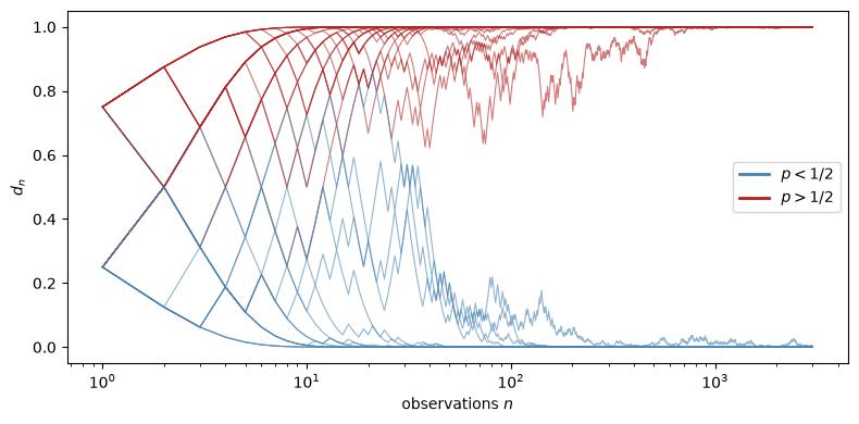
largest |d_n - 1{p > 1/2}| at n = 3000: 0.0034, on the path with p = 0.486
Every path ends near \(\mathbf{1}\{p > \tfrac12\}\); the paths that converge slowly have \(p\) near \(\tfrac12\).
Part 4.
With \(Q = P_1\) and \(P = P_2\), the hypothesis \(Q \ll P\) holds, and the theorem gives \(d_n \to 0\) \(P_1\)-a.s.
Because \(dP_1/dP_2 = 2\cdot\mathbf{1}\{\bar p < \tfrac12\}\), \(P_1\) is \(P_2\) conditioned on \(\{\bar p < \tfrac12\}\).
So the theorem’s conclusion is \(d_n \to 0\) \(P_2\)-a.s. on \(\{\bar p < \tfrac12\}\).
The theorem is silent on \(\{\bar p > \tfrac12\}\), an event with \(P_2\)-probability \(\tfrac12\) and \(P_1\)-probability zero.
There \(d_n \to 1\): agent 1’s prior rules out \(p > \tfrac12\), and no data move agent 1’s posterior mass above \(\tfrac12\).
Exercise 34.3
Let \(P = \mathcal{N}(0,1)^{\otimes \mathbb{N}}\) and \(Q = \bigotimes_m \mathcal{N}(\mu_m, 1)\), as in the Gaussian product-measure example, and let \(\sigma_n^2 = \sum_{m > n} \mu_m^2\).
Show that \(d_n = 2\Phi(\sigma_n/2) - 1\), with \(d_n = 1\) when \(\sigma_n = \infty\).
For \(\mu_m = c/m\), show that \(d_n \approx c/\sqrt{2\pi n}\) for large \(n\). Compare the exact and approximate values at \(n = 100\) with \(c = 2\).
For \(\mu_m = c/\sqrt{m}\), show that \(d_n = 1\) for every \(n\), while the distance between the two agents’ one-step-ahead forecasts, \(\|\mathcal{N}(0,1) - \mathcal{N}(\mu_{n+1}, 1)\|_{\mathrm{TV}}\), converges to zero.
Kalai and Lehrer [1994] call convergence of forecasts over every fixed finite horizon weak merging and convergence of \(d_n\) strong merging.
Part 3 gives weak merging without strong merging.
Solution
Part 1.
For product measures, the future is independent of the past, so \(d_n\) is the TV distance between \(\bigotimes_{m>n} \mathcal{N}(0,1)\) and \(\bigotimes_{m>n} \mathcal{N}(\mu_m,1)\).
Suppose \(\sigma_n < \infty\).
Then \(\sum_{m>n} (1 - \rho_m) \leq \sum_{m>n} \mu_m^2/8 < \infty\), so the two tail products are equivalent, and their likelihood ratio is
Under \(P\), \(S \sim \mathcal{N}(0, \sigma_n^2)\); under \(Q\), \(S \sim \mathcal{N}(\sigma_n^2, \sigma_n^2)\).
Because \(L\) is a function of \(S\), the TV distance between the tail products equals the TV distance between the two laws of \(S\).
Those two normal densities cross at \(\sigma_n^2/2\), so
Suppose \(\sigma_n = \infty\).
If \(\mu_m \not\to 0\), the terms \(1 - \rho_m = 1 - e^{-\mu_m^2/8}\) do not vanish; if \(\mu_m \to 0\), then \(1 - \rho_m \geq \mu_m^2/16\) for large \(m\).
Either way \(\sum_{m>n}(1-\rho_m) = \infty\), Kakutani’s theorem makes the tail products singular, and \(d_n = 1\).
Part 2.
For \(\mu_m = c/m\), \(\sigma_n^2 = c^2 \sum_{m>n} m^{-2}\), and \(1/(n+1) \leq \sum_{m>n} m^{-2} \leq 1/n\).
So \(\sigma_n \approx c/\sqrt{n}\), and \(2\Phi(x) - 1 \approx x\sqrt{2/\pi}\) for small \(x\) gives \(d_n \approx c/\sqrt{2\pi n}\).
The tail sum \(\sum_{m>n} m^{-2}\) is the trigamma function \(\psi'(n+1)\), which polygamma(1, n + 1) computes.
Part 3.
For \(\mu_m = c/\sqrt{m}\), \(\sum_{m>n} c^2/m = \infty\) for every \(n\), so \(d_n = 1\).
The one-step forecast distance is \(2\Phi(c/(2\sqrt{n+1})) - 1 \to 0\).
For any fixed \(k\), the distance between the two agents’ forecasts of \((x_{n+1}, \ldots, x_{n+k})\) is \(2\Phi\bigl(\tfrac12 (\sum_{m=n+1}^{n+k} c^2/m)^{1/2}\bigr) - 1 \leq 2\Phi\bigl(c\sqrt{k}/(2\sqrt{n+1})\bigr) - 1 \to 0\).
The agents’ forecasts of any fixed number of future observations merge, but their forecasts of the entire future never do.
c = 2.0
n_vals = np.arange(1, 1001)

σ_inv_m = c * np.sqrt(polygamma(1, n_vals + 1))     # μ_m = c/m
d_inv_m = 2 * norm.cdf(σ_inv_m / 2) - 1
d_inv_m_approx = c / np.sqrt(2 * np.pi * n_vals)
one_step_sqrt = 2 * norm.cdf(c / (2 * np.sqrt(n_vals + 1))) - 1   # μ_m = c/√m

fig, ax = plt.subplots(figsize=(8, 4))
ax.loglog(n_vals, d_inv_m, color='steelblue', lw=2,
          label=r'$d_n$, $\mu_m = c/m$')
ax.loglog(n_vals, d_inv_m_approx, color='steelblue', lw=1.5, ls='--',
          label=r'$c/\sqrt{2\pi n}$')
ax.loglog(n_vals, np.ones_like(n_vals, dtype=float), color='purple',
          lw=2, label=r'$d_n$, $\mu_m = c/\sqrt{m}$')
ax.loglog(n_vals, one_step_sqrt, color='purple', lw=1.5, ls=':',
          label=r'one-step distance, $\mu_m = c/\sqrt{m}$')
ax.set_xlabel('$n$')
ax.set_ylabel('total-variation distance')
ax.legend(fontsize=8)
plt.tight_layout()
plt.show()

n = 100
print(f"n = {n}: exact d_n = {d_inv_m[n - 1]:.4f}, "
      f"approximation = {d_inv_m_approx[n - 1]:.4f}")
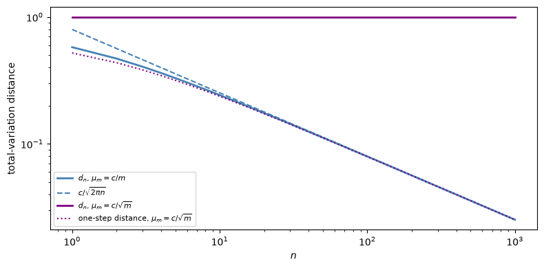
n = 100: exact d_n = 0.0795, approximation = 0.0798
At \(n = 100\) with \(c = 2\), the exact distance is \(0.0795\) and the approximation is \(0.0798\).
The one-step distance for \(\mu_m = c/\sqrt{m}\) nearly coincides with \(d_n\) for \(\mu_m = c/m\), because \(\mu_{n+1}^2 = c^2/(n+1)\) and \(c^2 \sum_{m>n} m^{-2}\) are both close to \(c^2/n\).
Exercise 34.4
Let \(\pi_1\) and \(\pi_2\) be prior densities on \((0,1)\) with \(\pi_2 > 0\) wherever \(\pi_1 > 0\), let \(P_i = \int_0^1 P_p\,\pi_i(p)\,dp\), and let \(\bar p = \limsup_n k_n/n\).
Show that \(dP_1/dP_2 = \pi_1(\bar p)/\pi_2(\bar p)\) on \(\mathscr{F}\), so that \(Z_\infty = \pi_1(\bar p)/\pi_2(\bar p)\).
For the priors \(\mathrm{Beta}(1,8)\) and \(\mathrm{Beta}(8,1)\), simulate several paths from \(P_2\). Compare \(\log Z_n\) at large \(n\) with \(7\log((1-\hat p_n)/\hat p_n)\), where \(\hat p_n = k_n/n\), and with \(7\log((1-p)/p)\), where \(p\) is the coin drawn on that path.
Solution
Part 1.
Under \(P_p\), the strong law of large numbers gives \(\bar p = p\) almost surely.
Set \(\pi_1/\pi_2 = 0\) where \(\pi_2 = 0\).
For every \(A \in \mathscr{F}\),
The second equality uses \(\pi_2 > 0\) wherever \(\pi_1 > 0\).
The third replaces \(p\) with \(\bar p\), which equals \(p\) \(P_p\)-a.s.
So \(\pi_1(\bar p)/\pi_2(\bar p)\) is a density of \(P_1\) with respect to \(P_2\) on \(\mathscr{F}\), and Lemma 34.1 gives \(Z_\infty = \pi_1(\bar p)/\pi_2(\bar p)\).
A Laplace approximation explains the convergence of \(Z_n\).
The ratio \(Z_n = \int_0^1 p^{k_n}(1-p)^{n-k_n}\pi_1(p)\,dp \,/\, \int_0^1 p^{k_n}(1-p)^{n-k_n}\pi_2(p)\,dp\) weights both priors by a likelihood that concentrates near \(\hat p_n\), so \(Z_n \approx \pi_1(\hat p_n)/\pi_2(\hat p_n)\).
Part 2.
n_ex = 20_000
rng_z = np.random.default_rng(5)

print(f"{'p':>6} {'p_hat':>7} {'log Z_n':>9} "
      f"{'gap to p_hat formula':>21} {'gap to p formula':>17}")
for j in range(6):
    p = rng_z.beta(a2, b2)                     # p drawn from π_2
    data = rng_z.binomial(1, p, n_ex)
    log_Z_n = log_likelihood_ratio(data, a1, b1, a2, b2)[-1]
    p_hat = data.mean()
    gap_hat = log_Z_n - 7 * np.log((1 - p_hat) / p_hat)
    gap_true = log_Z_n - 7 * np.log((1 - p) / p)
    print(f"{p:6.3f} {p_hat:7.4f} {log_Z_n:9.3f} "
          f"{gap_hat:21.3f} {gap_true:17.3f}")
     p   p_hat   log Z_n  gap to p_hat formula  gap to p formula
 0.813  0.8105   -10.169                 0.006             0.113
 0.918  0.9191   -16.996                 0.016            -0.057
 0.877  0.8740   -13.545                 0.009             0.211
 0.917  0.9141   -16.534                 0.015             0.254
 0.856  0.8536   -12.334                 0.008             0.118
 0.986  0.9862   -29.811                 0.099             0.199
At \(n = 20{,}000\), \(\log Z_n\) differs from \(7\log((1-\hat p_n)/\hat p_n)\) by at most \(0.10\) across these paths.
That gap is the \(O(1/n)\) error of the Laplace approximation, and it is largest on the path with \(p\) closest to one, where the derivatives of \(\log(\pi_1/\pi_2)\) are large.
The gap between \(\log Z_n\) and \(7\log((1-p)/p)\) reaches \(0.25\), because \(\hat p_n\) differs from \(p\) by \(O(n^{-1/2})\); that gap vanishes as \(\hat p_n \to p\).
On the path in the first figure of the lecture, \(\log Z_{600} = -4.07\) and \(7\log((1-\hat p_{600})/\hat p_{600}) = -4.13\).