28. Exchangeability and Bayesian Updating#
28.1. Overview#
This lecture studies learning via Bayes’ Law.
We touch foundations of Bayesian statistical inference invented by de Finetti [1937].
The relevance of de Finetti’s work for economists is presented forcefully by David Kreps in chapter 11 of [Kreps, 1988].
An example that we study below is a key component of Job Search IX: Search with Learning.
That lecture augments the classic job search model of McCall [McCall, 1970], studied in Job Search I: The McCall Search Model, by presenting an unemployed worker with a statistical inference problem.
Here we create graphs that illustrate the role that a likelihood ratio plays in Bayes’ Law.
We’ll use such graphs to provide insights into the mechanics driving outcomes in Job Search IX: Search with Learning.
Among other things, this lecture discusses connections between the statistical concepts of sequences of random variables that are
independently and identically distributed
exchangeable
Understanding these concepts is essential for appreciating how Bayesian updating works.
You can read about exchangeability here.
De Finetti’s theorem states that an infinite exchangeable sequence is conditionally independently and identically distributed: it is IID conditional on a random variable whose value the observer does not know.[1]
We want to convey an answer to the question conditional on what?
We also tell why an assumption of independence precludes learning while an assumption that a sequence is conditionally IID makes learning possible.
Below, we’ll often use
\(W\) to denote a random variable
\(w\) to denote a particular realization of a random variable \(W\)
Let’s start with some imports:
from math import gamma

import matplotlib.pyplot as plt
import numpy as np
import scipy.optimize as op
from scipy.integrate import quad
from scipy.special import expit
28.2. Independently and identically distributed#
We begin by looking at the notion of an independently and identically distributed sequence of random variables.
An independently and identically distributed sequence is often abbreviated as IID.
Two notions are involved
independence
identically distributed
A sequence \(W_0, W_1, \ldots\) is independently distributed if, for every \(n \geq 0\), the joint probability density of \(W_0, W_1, \ldots, W_n\) is the product of the marginal densities of \(W_0, W_1, \ldots, W_n\).
The sequence \(W_0, W_1, \ldots\) is independently and identically distributed (IID) if in addition the marginal density of \(W_t\) is the same for all \(t =0, 1, \ldots\).
For example, let \(p(W_0, W_1, \ldots, W_n)\) be the joint density of \(W_0, W_1, \ldots, W_n\) and let \(p(W_t)\) be the common marginal density of each \(W_t\).
Then the sequence \(W_0, W_1, \ldots\) is IID if
so that each joint density is the product of identical marginal densities.
28.2.1. IID means past observations don’t tell us anything about future observations#
If a sequence of random variables is IID, past information provides no information about future realizations.
Therefore, there is nothing to learn from the past about the future.
To understand these statements, let the joint distribution of a sequence of random variables \(\{W_t\}_{t=0}^T\) that is not necessarily IID be
Using the laws of probability, we can always factor such a joint density into a product of conditional densities:
In general,
which states that the conditional density on the left side does not equal the marginal density on the right side.
But in the special IID case,
so that the partial history \(W_{t-1}, \ldots, W_0\) contains no information about the probability of \(W_t\).
So in the IID case, there is nothing to learn about the densities of future random variables from past random variables.
But when the sequence is not IID, there is something to learn about the future from observations of past random variables.
We turn next to an instance of the general case in which the sequence is not IID.
Please watch for what can be learned from the past and when.
28.3. A setting in which past observations are informative#
Let \(\{W_t\}_{t=0}^\infty\) be a sequence of nonnegative scalar random variables with a joint probability distribution constructed as follows.
There are two distinct cumulative distribution functions \(F\) and \(G\) that have densities \(f\) and \(g\), respectively, for a nonnegative scalar random variable \(W\).
Before the start of time, say at time \(t= -1\), “nature” once and for all selects either \(f\) or \(g\).
Thereafter at each time \(t \geq 0\), nature draws a random variable \(W_t\) from the selected distribution.
So the data are permanently generated as independently and identically distributed (IID) draws from either \(F\) or \(G\).
We could say that objectively, meaning after nature has chosen either \(F\) or \(G\), the probability that the data are generated as draws from \(F\) is either \(0\) or \(1\).
We now drop into this setting a partially informed decision maker who
knows both \(F\) and \(G\), but
does not know whether at \(t = -1\) nature had drawn \(F\) or whether nature had drawn \(G\) once-and-for-all
Thus, although our decision maker knows \(F\) and knows \(G\), he does not know which of these two known distributions nature had selected to draw from.
The decision maker describes his ignorance with a subjective probability \(\tilde \pi\) and reasons as if nature had selected \(F\) with probability \(\tilde \pi \in (0,1)\) and \(G\) with probability \(1 - \tilde \pi\).
Thus, we assume that the decision maker
knows both \(F\) and \(G\)
doesn’t know which of these two distributions that nature has drawn
expresses his ignorance by acting as if or thinking that nature chose distribution \(F\) with probability \(\tilde \pi \in (0,1)\) and distribution \(G\) with probability \(1 - \tilde \pi\)
at date \(t \geq 0\) knows the partial history \(w_t, w_{t-1}, \ldots, w_0\)
To proceed, we want to know the decision maker’s belief about the joint distribution of the partial history.
We’ll discuss that next and in the process describe the concept of exchangeability.
28.4. Relationship between IID and exchangeable#
Conditional on nature selecting \(F\), the joint density of \(W_0, W_1, \ldots, W_n\) is
for every \(n \geq 0\).
Conditional on nature selecting \(G\), the joint density of \(W_0, W_1, \ldots, W_n\) is
Thus, conditional on nature having selected \(F\), the sequence \(W_0, W_1, \ldots\) is independently and identically distributed.
Furthermore, conditional on nature having selected \(G\), the sequence \(W_0, W_1, \ldots\) is also independently and identically distributed.
But what about the unconditional distribution of a partial history?
The unconditional joint density of \(W_0, W_1, \ldots, W_n\) is evidently
Under the unconditional distribution (28.1), the sequence \(W_0, W_1, \ldots\) is not independently and identically distributed.
To verify this claim, let \(h(W_t) = \tilde \pi f(W_t) + (1-\tilde \pi) g(W_t)\) be the marginal density of \(W_t\).
Then
The right side is not zero when \(f(W_0) \neq g(W_0)\) and \(f(W_1) \neq g(W_1)\), so the joint density \(h(W_0, W_1)\) is not the product of the marginal densities \(h(W_0)\) and \(h(W_1)\).
Thus, the conditional distribution
This means that random variable \(W_0\) contains information about random variable \(W_1\).
So there is something to learn from the past about the future.
Exercise Exercise 28.1 uses (28.2) to show that \(W_0\) and \(W_1\) are positively correlated.
28.5. Exchangeability#
While the sequence \(W_0, W_1, \ldots\) is not IID, it can be verified that it is exchangeable, which means that the joint distributions \(h(W_0, W_1)\) and \(h(W_1, W_0)\) of the “re-ordered” sequences satisfy
and so on.
More generally, a sequence of random variables is said to be exchangeable if the joint probability distribution for a sequence does not change when the positions in the sequence in which finitely many of random variables appear are altered.
Equation (28.1) represents our instance of an exchangeable joint density over a sequence of random variables as a mixture of two IID joint densities over a sequence of random variables.
A Bayesian statistician interprets the mixing parameter \(\tilde \pi \in (0,1)\) as a decision maker’s subjective belief – the decision maker’s prior probability – that nature had selected probability distribution \(F\).
28.5.1. De Finetti’s theorem#
As de Finetti [1937] proved, every infinite exchangeable sequence is a mixture of IID sequences.
For binary random variables \(W_t \in \{0, 1\}\), de Finetti’s theorem states that the infinite sequence \(W_0, W_1, \ldots\) is exchangeable if and only if there is a probability measure \(\mu\) on \([0,1]\) such that
for every \(n \geq 1\) and every \((w_0, \ldots, w_{n-1}) \in \{0,1\}^n\).
The mixing measure \(\mu\) is unique.
It is the probability distribution of the limiting relative frequency
a limit that exists with probability one.
Conditional on \(\theta\), the \(W_t\) are IID Bernoulli random variables with success probability \(\theta\).
This answers the question conditional on what?: conditional on the limiting relative frequency \(\theta\).
A Bayesian statistician interprets \(\mu\) as a prior probability distribution over the unknown Bernoulli parameter \(\theta \in [0,1]\).
The measure \(\mu\) need not have a density; it can put positive probability on finitely many points.
Hewitt and Savage [1955] extended de Finetti’s theorem to sequences that take values in more general spaces.
In their version the mixing measure is a probability distribution over probability distributions of \(W\), and the conditioning variable is the limiting empirical distribution of \(W_0, W_1, \ldots\).
Equation (28.1) is an instance with a two-point mixing measure that puts probability \(\tilde \pi\) on \(F\) and probability \(1 - \tilde \pi\) on \(G\).
In that instance the limiting empirical distribution of \(W_0, W_1, \ldots\) is \(F\) when nature has drawn \(F\) and \(G\) when nature has drawn \(G\).
De Finetti’s theorem requires an infinite sequence.
Exercise Exercise 28.1 describes a finite exchangeable sequence that is not a mixture of IID sequences.
The Beta–Bernoulli model in Merging of Opinions: The Blackwell–Dubins Theorem is the instance of (28.3) in which \(\mu\) is a Beta distribution.
Exercise Exercise 28.3 describes an urn scheme that generates it.
28.6. Bayes’ Law#
We noted above that in our example model there is something to learn about the future from past data drawn from our particular instance of a process that is exchangeable but not IID.
But how can we learn?
And about what?
The answer to the about what question is: about which distribution, \(F\) or \(G\), nature selected at time \(-1\).
The decision maker knows his prior probability \(\tilde \pi\).
What he learns is expressed in a posterior probability that moves away from \(\tilde \pi\) as data arrive.
The answer to the how question is to use Bayes’ Law.
Another way to say use Bayes’ Law is to say from a (subjective) joint distribution, compute an appropriate conditional distribution.
Let’s dive into Bayes’ Law in this context.
Let \(q\) represent the distribution that nature actually draws \(w\) from and let
where we regard \(\pi\) as a decision maker’s subjective probability (also called a personal probability).
Suppose that at \(t \geq 0\), the decision maker has observed a history \(w^t \equiv [w_t, w_{t-1}, \ldots, w_0]\).
We let
where we adopt the convention
Conditional on \(q\), the draw \(w_{t+1}\) is independent of the history \(w^t\).
The density of \(w_{t+1}\) conditional on \(w^t\) is then
Bayes’ rule for updating \(\pi_{t+1}\) is
Equation (28.4) follows from Bayes’ rule, which tells us that
where \(p\) denotes a density and
Because \(w_{t+1}\) is independent of \(w^t\) conditional on \(q\), \(p(w_{t+1} \,|\, q = f, w^t) = f(w_{t+1})\) and \(p(w_{t+1} \,|\, q = g, w^t) = g(w_{t+1})\).
28.7. More details about Bayesian updating#
Let’s stare at and rearrange Bayes’ Law as represented in equation (28.4) with the aim of understanding how the posterior probability \(\pi_{t+1}\) is influenced by the prior probability \(\pi_t\) and the likelihood ratio
It is convenient for us to rewrite the updating rule (28.4) as
This implies that
The likelihood ratio alone determines whether an observation \(w_{t+1}\) leads the decision maker to increase or decrease the subjective probability he/she attaches to distribution \(F\).
When the likelihood ratio \(\ell(w_{t+1})\) exceeds one, the observation \(w_{t+1}\) nudges the probability \(\pi\) put on distribution \(F\) upward, and when the likelihood ratio \(\ell(w_{t+1})\) is less than one, the observation \(w_{t+1}\) nudges \(\pi\) downward.
The prior \(\pi_t\) affects the size of the move:
The move shrinks to zero as \(\pi_t\) approaches \(0\) or \(1\).
Representation (28.5) is the foundation of some graphs that we’ll use to display the dynamics of \(\{\pi_t\}_{t=0}^\infty\) that are induced by Bayes’ Law.
We’ll plot \(\ell\left(w\right)\) as a way to enlighten us about how learning – i.e., Bayesian updating of the probability \(\pi\) that nature has chosen distribution \(f\) – works.
We build up the picture in three steps, each of which produces one graph.
All three are built from the same ingredients: the densities \(f\) and \(g\), and the values of \(w\) at which the likelihood ratio \(\ell(w) = f(w)/g(w)\) crosses one.
Both \(f\) and \(g\) are Beta densities, so we start with the general Beta density.
def p(w, a, b):
    "The Beta density with parameters a and b."
    r = gamma(a + b) / (gamma(a) * gamma(b))
    return r * w**(a - 1) * (1 - w)**(b - 1)
The next function assembles the ingredients for a given pair of Beta distributions.
def create_model(F_a=1, F_b=1, G_a=3, G_b=1.2):
    """
    Build the densities f and g, along with the two values of w at which
    the likelihood ratio ℓ(w) = f(w) / g(w) equals one.

    The root finder assumes that f is uniform (F_a = F_b = 1) and that
    G_a > 1 and G_b > 1.  Then g vanishes at 0 and 1 and has a single
    interior mode at which g exceeds one, so ℓ(w) = 1 / g(w) equals one
    exactly once on each side of the mode of g.
    """
    f = lambda w: p(w, F_a, F_b)
    g = lambda w: p(w, G_a, G_b)

    # The mode of g divides [0, 1] into two intervals, each holding one root
    G_mode = (G_a - 1) / (G_a + G_b - 2)
    obj = lambda w: f(w) / g(w) - 1
    roots = np.array([op.root_scalar(obj, bracket=[1e-10, G_mode]).root,
                      op.root_scalar(obj, bracket=[G_mode, 1 - 1e-10]).root])
    return f, g, roots
28.7.1. The likelihood ratio#
Our first graph plots the likelihood ratio \(\ell(w)\) on the abscissa axis against \(w\) on the ordinate axis.
We orient it this way so that \(w\) shares an axis with the two graphs that follow.
def plot_likelihood_ratio(F_a=1, F_b=1, G_a=3, G_b=1.2):
    f, g, roots = create_model(F_a, F_b, G_a, G_b)
    w_grid = np.linspace(1e-12, 1 - 1e-12, 100)

    fig, ax = plt.subplots(figsize=(6, 5))
    ax.plot(f(w_grid) / g(w_grid), w_grid, label=r'$\ell$', lw=2)
    ax.vlines(1, 0, 1, linestyle='--')
    ax.hlines(roots, 0, 2, linestyle='--')
    ax.set_xlim(0, 2)
    ax.legend(loc=4)
    ax.set(xlabel=r'$\ell(w) = f(w) / g(w)$', ylabel='$w$')
    plt.show()
We begin with \(f\) uniform on \([0,1]\) — that is, Beta with \(F_a=1, F_b=1\) — and \(g\) Beta with \(G_a=3, G_b=1.2\).
plot_likelihood_ratio()
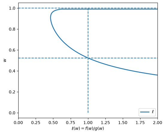
The two horizontal dashed lines mark the values of \(w\) at which \(\ell(w) = 1\).
Between them the likelihood ratio is below one, so by (28.5) a draw in that region pushes \(\pi\) down.
Outside them it exceeds one, so a draw there pushes \(\pi\) up.
28.7.2. The densities and the probabilities of moving in each direction#
Our second graph plots \(f(w)\) and \(g(w)\) against \(w\), and shades the regions delineated by those same two values of \(w\).
Shading them lets us attach a probability to each direction of movement, which we compute by integrating the relevant density over the region.
def plot_densities(F_a=1, F_b=1, G_a=3, G_b=1.2):
    f, g, roots = create_model(F_a, F_b, G_a, G_b)
    w_grid = np.linspace(0, 1, 100)

    fig, ax = plt.subplots(figsize=(6, 5))
    ax.plot(f(w_grid), w_grid, label='$f$', lw=2)
    ax.plot(g(w_grid), w_grid, label='$g$', lw=2)
    ax.vlines(1, 0, 1, linestyle='--')
    ax.hlines(roots, 0, 2, linestyle='--')
    ax.legend(loc=4)
    ax.set(xlabel='$f(w), g(w)$', ylabel='$w$')

    # Probability of landing in each region, under whichever density is shaded
    area_lower = quad(f, 0, roots[0])[0]
    area_middle = quad(g, roots[0], roots[1])[0]
    area_upper = quad(f, roots[1], 1)[0]

    ax.fill_between([0, 1], 0, roots[0], color='blue', alpha=0.15)
    ax.text((f(0) + f(roots[0])) / 4, roots[0] / 2, f"{area_lower: .3g}")
    w_middle = np.linspace(roots[0], roots[1], 20)
    ax.fill_betweenx(w_middle, 0, g(w_middle), color='orange', alpha=0.15)
    ax.text(np.mean(g(roots)) / 2, np.mean(roots), f"{area_middle: .3g}")
    ax.fill_between([0, 1], roots[1], 1, color='blue', alpha=0.15)
    ax.text((f(roots[1]) + f(1)) / 4, (roots[1] + 1) / 2, f"{area_upper: .3g}")
    plt.show()
Let’s look at the same pair of distributions as before.
plot_densities()
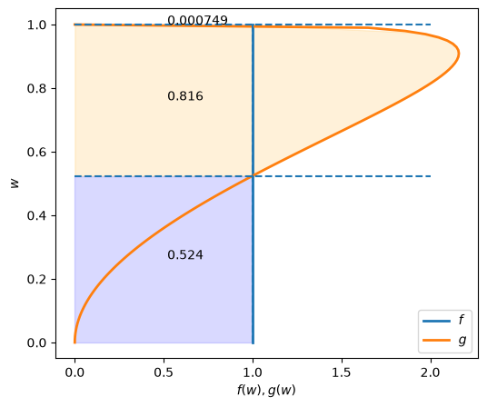
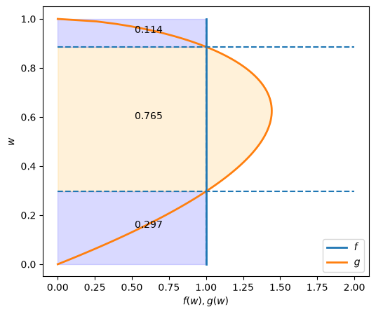
The fractions in the colored areas are probabilities that a realization of \(w\) falls into the region beside them.
The blue regions are integrals of \(f\) and the orange region is an integral of \(g\).
For example, under true distribution \(F\), \(\pi\) will be updated toward \(0\) if \(w\) falls into the interval \([0.524, 0.999]\), which occurs with probability \(0.999 - 0.524 \approx 0.475\) under \(F\).
But this would occur with probability \(0.816\) if \(G\) were the true distribution.
28.7.3. Dynamics of the belief#
Our third graph attaches an arrow to each point in the \((\pi, w)\) plane showing the change in \(\pi\) that Bayes’ Law induces when the current belief is \(\pi\) and the new draw is \(w\).
def plot_belief_dynamics(F_a=1, F_b=1, G_a=3, G_b=1.2):
    f, g, roots = create_model(F_a, F_b, G_a, G_b)
    π_grid = np.linspace(1e-3, 1 - 1e-3, 100)

    # Change in π at each point of a coarse grid over (π, w)
    W = np.arange(0.01, 0.99, 0.08)
    Π = np.arange(0.01, 0.99, 0.08)
    lw = (f(W) / g(W))[:, None]     # likelihood ratio at each w, as a column
    ΔΠ = Π * (lw / (Π * lw + 1 - Π) - 1)
    ΔW = np.zeros_like(ΔΠ)

    fig, ax = plt.subplots(figsize=(6, 5))
    ax.quiver(Π, W, ΔΠ, ΔW, scale=2, color='r', alpha=0.8)
    ax.fill_between(π_grid, 0, roots[0], color='blue', alpha=0.15)
    ax.fill_between(π_grid, roots[0], roots[1], color='green', alpha=0.15)
    ax.fill_between(π_grid, roots[1], 1, color='blue', alpha=0.15)
    ax.hlines(roots, 0, 1, linestyle='--')
    ax.set(xlabel=r'$\pi$', ylabel='$w$')
    ax.grid()
    plt.show()
Again we use the same pair of distributions.
plot_belief_dynamics()
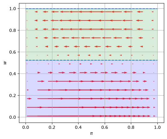
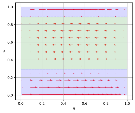
Arrows pointing right show when Bayes’ Law makes \(\pi\) increase and arrows pointing left show when it makes \(\pi\) decrease.
Lengths of the arrows show magnitudes of the force from Bayes’ Law impelling \(\pi\) to change.
These lengths depend on both the prior probability \(\pi\) on the abscissa axis and the evidence in the form of the current draw of \(w\) on the ordinate axis.
Arrows point right in the blue regions, where \(\ell(w) > 1\), and left in the green region between the dashed lines, where \(\ell(w) < 1\).
For these parameters the upper blue region is a thin sliver just below \(w = 1\), since \(\ell(w)\) returns above one only for draws very close to the upper limit.
28.7.4. Another instance#
Next we use our code to create graphs for another instance of our model.
We keep \(F\) the same as in the preceding instance, namely a uniform distribution, but now assume that \(G\) is a Beta distribution with parameters \(G_a=2, G_b=1.6\).
plot_likelihood_ratio(G_a=2, G_b=1.6)
plot_densities(G_a=2, G_b=1.6)
plot_belief_dynamics(G_a=2, G_b=1.6)
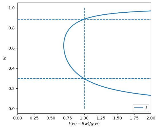
Notice how the likelihood ratio, the densities, and the arrows compare with the previous instance of our example.
28.8. Appendix#
28.8.1. Sample paths of \(\pi_t\)#
Now we’ll have some fun by plotting multiple realizations of sample paths of \(\pi_t\) under two possible assumptions about nature’s choice of distribution, namely
that nature permanently draws from \(F\)
that nature permanently draws from \(G\)
Outcomes depend on a peculiar property of likelihood ratio processes discussed in this section of Likelihood Ratio Processes.
Before simulating, it pays to rewrite Bayes’ Law in terms of odds rather than probabilities.
In terms of the odds \(\pi / (1 - \pi)\), the updating rule (28.4) becomes
So Bayes’ Law is multiplicative in the odds, and iterating (28.6) back to the prior \(\pi_{-1}\) yields
The belief path is thus a running product of likelihood ratios, which is why properties of likelihood ratio processes govern its behavior.
Taking logarithms turns the product into a sum:
We simulate with this sum.
It avoids overflow in the product and loss of precision when \(\pi_t\) is close to \(0\) or \(1\).
It also means that we can simulate an entire ensemble of paths with a cumulative sum, with no iteration over dates.
def simulate(rng, a, b, T=50, N=1000, π_init=0.5,
             F_a=1, F_b=1, G_a=3, G_b=1.2):
    """
    Simulate N paths of the belief π when nature draws w_0, ..., w_{T-1}
    IID from Beta(a, b).  Returns an array of shape (N, T+1) whose column 0
    holds the prior π_{-1} = π_init and whose column t+1 holds π_t.
    """
    w = rng.beta(a, b, size=(N, T))
    log_l = np.log(p(w, F_a, F_b)) - np.log(p(w, G_a, G_b))
    log_odds = np.log(π_init / (1 - π_init)) + np.cumsum(log_l, axis=1)
    return np.column_stack([np.full(N, π_init), expit(log_odds)])
The paths are plotted by the next function.
def plot_paths(π_paths):
    "Plot belief paths against the dates t = -1, 0, ..., T-1."
    t = np.arange(π_paths.shape[1]) - 1
    fig, ax = plt.subplots()
    ax.plot(t, π_paths.T, color='b', lw=0.8, alpha=0.5)
    ax.set(xlabel='$t$', ylabel=r'$\pi_t$')
    plt.show()
We begin by generating \(N\) simulated \(\{\pi_t\}\) paths with \(T\) periods when the sequence is truly IID draws from \(F\). We set an initial prior \(\pi_{-1} = .5\).
rng = np.random.default_rng(42)
T = 50
# when nature selects F
π_paths_F = simulate(rng, a=1, b=1, T=T, N=1000)
plot_paths(π_paths_F)
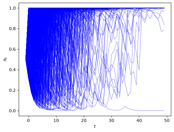
In the above example, for most paths \(\pi_t \rightarrow 1\).
So Bayes’ Law evidently eventually discovers the truth for most of our paths.
Next, we generate paths with \(T\) periods when the sequence is truly IID draws from \(G\). Again, we set the initial prior \(\pi_{-1} = .5\).
# when nature selects G
π_paths_G = simulate(rng, a=3, b=1.2, T=T, N=1000)
plot_paths(π_paths_G)
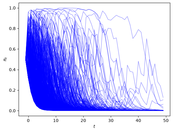
In the above graph we observe that now most paths \(\pi_t \rightarrow 0\).
28.8.2. Rates of convergence#
We study rates of convergence of \(\pi_t\) to \(1\) when nature generates the data as IID draws from \(F\) and of convergence of \(\pi_t\) to \(0\) when nature generates IID draws from \(G\).
We do this by averaging across simulated paths of \(\{\pi_t\}_{t=-1}^{T-1}\).
Using \(N\) simulated \(\pi_t\) paths, we compute \(1 - \frac{1}{N}\sum_{i=1}^{N}\pi_{i,t}\) at each \(t\) when the data are generated as draws from \(F\) and compute \(\frac{1}{N}\sum_{i=1}^{N}\pi_{i,t}\) when the data are generated as draws from \(G\).
t_grid = np.arange(-1, T)
fig, ax = plt.subplots()
ax.plot(t_grid, 1 - np.mean(π_paths_F, axis=0), label='F generates')
ax.plot(t_grid, np.mean(π_paths_G, axis=0), label='G generates')
ax.set(xlabel='$t$', title='convergence')
ax.legend()
plt.show()
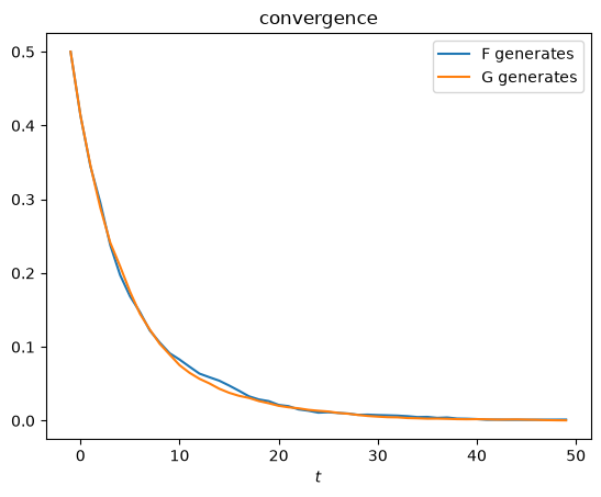
The two curves nearly coincide.
An exact identity explains why:
Here \(E_f\) and \(E_g\) denote expectations under IID draws from \(F\) and from \(G\), and \(E\) denotes the expectation under the decision maker’s subjective joint distribution (28.1).
To prove (28.8), let \(\phi\) be a bounded function of the history \(w^t\).
Because \(\pi_t = \mathbb{P}\{q = f \,|\, w^t\}\), the law of iterated expectations implies
Setting \(\phi = 1 - \pi_t\) equates the first and third terms of (28.8).
The same argument applied to \(1 - \pi_t = \mathbb{P}\{q = g \,|\, w^t\}\) with \(\phi = \pi_t\) equates the second and third terms.
With \(\pi_{-1} = 0.5\), the identity says that \(E_f[1 - \pi_t] = E_g[\pi_t]\) for every \(t\), so the two simulated curves differ only by sampling error.
With another prior, the two curves differ by the constant factor \((1 - \pi_{-1})/\pi_{-1}\).
The identity does not say that typical paths converge at the same rate under \(F\) and under \(G\).
By (28.7) and the law of large numbers, \(\frac{1}{t+1} \log \frac{\pi_t}{1 - \pi_t}\) converges to \(E_f[\log \ell(w)] = KL(f, g) = 0.759\) when \(F\) generates the data and to \(E_g[\log \ell(w)] = -KL(g, f) = -0.344\) when \(G\) generates the data, where \(KL(f, g) = \int f(w) \log \frac{f(w)}{g(w)} dw\) is the Kullback–Leibler divergence of \(g\) from \(f\).
So a typical path approaches \(1\) under \(F\) faster than it approaches \(0\) under \(G\).
The averages plotted above are dominated by rare paths along which \(\pi_t\) leans the wrong way for a long time.
Both averages decay at the exponential rate
the Chernoff entropy of \(f\) and \(g\) described in Statistical Divergence Measures.
Exercise Exercise 28.2 verifies these claims.
28.8.3. Graph of ensemble dynamics of \(\pi_t\)#
More insights about the dynamics of \(\{\pi_t\}\) can be gleaned by computing conditional expectations of \(\frac{\pi_{t+1}}{\pi_{t}}\) as functions of \(\pi_t\) via integration with respect to the pertinent probability distribution:
where \(a =f,g\).
The following code approximates the integral above:
def plot_expected_ratio(F_a=1, F_b=1, G_a=3, G_b=1.2):
    # Build f and g directly: here they can coincide, so ℓ(w) = 1 has no root
    f = lambda w: p(w, F_a, F_b)
    g = lambda w: p(w, G_a, G_b)
    l = lambda w: f(w) / g(w)
    π_grid = np.linspace(0.02, 0.98, 100)

    fig, ax = plt.subplots()
    for label, a in [('f', f), ('g', g)]:
        integrand = lambda w, π: a(w) * l(w) / (π * l(w) + 1 - π)
        ratios = [quad(integrand, 0, 1, args=(π,))[0] for π in π_grid]
        ax.plot(π_grid, ratios, label=f'{label} generates')

    ax.hlines(1, 0, 1, linestyle='--')
    ax.set(xlabel=r'$\pi_t$', ylabel=r'$E[\pi_{t+1} / \pi_t]$')
    ax.legend()
    plt.show()
First, consider the case where \(F_a=F_b=1\) and \(G_a=3, G_b=1.2\).
plot_expected_ratio()
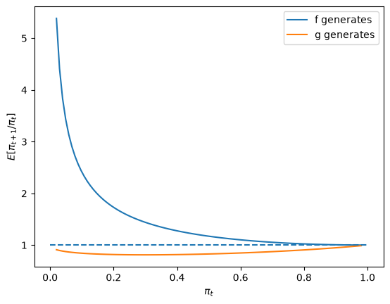
The above graph shows that when \(F\) generates the data, \(\pi_t\) on average always heads north, while when \(G\) generates the data, \(\pi_t\) heads south.
Two inequalities hold for every pair \(f \neq g\) and every \(\pi_t = \pi \in (0,1)\).
Let \(r(\ell) = \ell / (\pi \ell + 1 - \pi)\) be the ratio \(\pi_{t+1}/\pi_t\) as a function of \(\ell = \ell(w_{t+1})\).
The function \(r\) is strictly concave and \(E_g[\ell(w)] = \int f(w) dw = 1\), so Jensen’s inequality implies
The \(\pi\)-weighted average of the two expectations equals one:
This equality is the martingale property of \(\pi_t\) under the decision maker’s subjective distribution, studied in Likelihood Ratio Processes and Bayesian Learning.
It and the first inequality imply
Thus \(\pi_t\) is a submartingale when \(F\) generates the data and a supermartingale when \(G\) generates the data.
Next, we’ll look at a degenerate case in which \(f\) and \(g\) are identical beta distributions, and \(F_a=G_a=3, F_b=G_b=1.2\).
In a sense, here there is nothing to learn.
plot_expected_ratio(F_a=3, F_b=1.2)
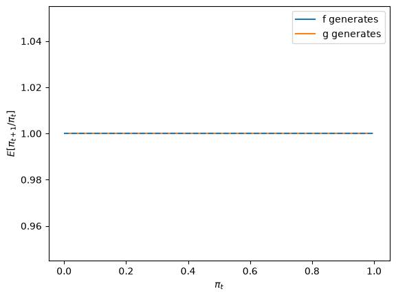
The above graph says that \(\pi_t\) is inert and remains at its initial value.
Finally, let’s look at a case in which \(f\) and \(g\) are neither very different nor identical, in particular one in which \(F_a=2, F_b=1\) and \(G_a=3, G_b=1.2\).
plot_expected_ratio(F_a=2, F_b=1, G_a=3, G_b=1.2)
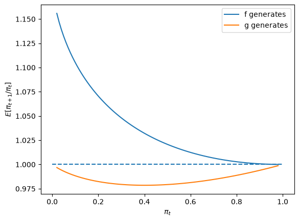
The two inequalities still hold, but both curves now stay close to one.
On the plotted grid, \(E_f[\pi_{t+1}/\pi_t]\) never exceeds \(1.16\) and \(E_g[\pi_{t+1}/\pi_t]\) never falls below \(0.978\).
In the first case the corresponding numbers are \(5.38\) and \(0.811\).
The densities Beta\((2,1)\) and Beta\((3,1.2)\) are close to each other: \(KL(f, g) = 0.052\) and \(KL(g, f) = 0.039\), compared with \(0.759\) and \(0.344\) in the first case.
A draw moves \(\pi_t\) only a little on average, so learning is slow.
28.9. Sequels#
We’ll apply and dig deeper into some of the ideas presented in this lecture:
Likelihood Ratio Processes describes likelihood ratio processes and their role in frequentist and Bayesian statistical theories
Likelihood Ratio Processes and Bayesian Learning studies how a likelihood ratio process drives the posterior probability \(\pi_t\) and shows that \(\pi_t\) is a martingale under the decision maker’s subjective distribution (28.1)
Incorrect Models studies a decision maker who uses this lecture’s statistical model when nature actually mixes \(F\) and \(G\) anew each period
Merging of Opinions: The Blackwell–Dubins Theorem studies the Beta–Bernoulli model, an instance of de Finetti’s representation (28.3), and asks when the opinions of two Bayesians with different priors merge
Statistical Divergence Measures describes the Kullback–Leibler divergence and the Chernoff entropy that govern rates of learning
A Bayesian Formulation of Friedman and Wald’s Problem studies a decision maker with this lecture’s beliefs who decides sequentially when to stop sampling
Bayesian versus Frequentist Decision Rules studies a World War II US Navy Captain’s hunch that a (frequentist) decision rule that the Navy had told him to use was inferior to a sequential rule that Abraham Wald had not yet designed
28.10. Exercises#
Exercise 28.1
This exercise shows that a mixture of IID sequences has nonnegative serial covariances and that a finite exchangeable sequence need not be a mixture of IID sequences.
Prove identity (28.2).
Let \(\phi\) be a function for which \(E_f[\phi(W)]\) and \(E_g[\phi(W)]\) are finite. Use (28.2) to show that under the joint density (28.1)
For this lecture’s densities \(f = \) Beta\((1, 1)\) and \(g = \) Beta\((3, 1.2)\) and \(\tilde \pi = 0.5\), compute \(\textrm{Cov}(W_0, W_1)\) from the formula in part 2 and compare it with a simulation.
An urn contains one red ball and one black ball. We draw both balls without replacement. Let \(W_t = 1\) if draw \(t \in \{0, 1\}\) is red and \(W_t = 0\) if it is black. Show that \((W_0, W_1)\) is exchangeable and that \(\textrm{Cov}(W_0, W_1) < 0\). Explain why \((W_0, W_1)\) is not a mixture of IID pairs and why de Finetti’s theorem requires an infinite sequence.
Solution
Part 1.
With \(h(W_t) = \tilde \pi f(W_t) + (1 - \tilde \pi) g(W_t)\),
Subtracting this from \(h(W_0, W_1) = \tilde \pi f(W_0) f(W_1) + (1 - \tilde \pi) g(W_0) g(W_1)\) and using \(\tilde \pi - \tilde \pi^2 = (1 - \tilde \pi) - (1 - \tilde \pi)^2 = \tilde \pi (1 - \tilde \pi)\) gives
which factors into the right side of (28.2).
Part 2.
Multiply (28.2) by \(\phi(W_0) \phi(W_1)\) and integrate over \(W_0\) and \(W_1\):
The same conclusion holds for a mixture of IID sequences with any mixing measure.
Let \(Q\) be the distribution, drawn from the mixing measure, from which the \(W_t\) are IID draws.
The law of total covariance gives
Part 3.
The means of Beta\((1,1)\) and Beta\((3, 1.2)\) are \(1/2\) and \(3/4.2\).
π_tilde = 0.5
μ_f, μ_g = 1 / (1 + 1), 3 / (3 + 1.2)
cov_theory = π_tilde * (1 - π_tilde) * (μ_f - μ_g)**2

rng = np.random.default_rng(1234)
N = 1_000_000
nature_draws_f = rng.random(N) < π_tilde
W = np.where(nature_draws_f[:, None],
             rng.beta(1, 1, size=(N, 2)),
             rng.beta(3, 1.2, size=(N, 2)))
cov_sim = np.cov(W[:, 0], W[:, 1])[0, 1]

print(f"Cov(W_0, W_1): formula {cov_theory:.5f}, simulation {cov_sim:.5f}")
Cov(W_0, W_1): formula 0.01148, simulation 0.01147
Part 4.
The first draw is red with probability \(1/2\), and then the second draw is black with probability one.
So \(\textrm{Prob}(W_0 = 1, W_1 = 0) = \textrm{Prob}(W_0 = 0, W_1 = 1) = 1/2\) and \(\textrm{Prob}(W_0 = W_1) = 0\).
The joint distribution is invariant to exchanging \(W_0\) and \(W_1\), so \((W_0, W_1)\) is exchangeable.
\(E[W_0] = E[W_1] = 1/2\) and \(E[W_0 W_1] = 0\), so \(\textrm{Cov}(W_0, W_1) = -1/4\).
By part 2, every mixture of IID pairs has \(\textrm{Cov}(W_0, W_1) \geq 0\).
So \((W_0, W_1)\) is not a mixture of IID pairs.
If \((W_0, W_1)\) were the first two members of an infinite exchangeable sequence, de Finetti’s theorem would make the pair a mixture of IID pairs.
So the urn sequence cannot be extended to an infinite exchangeable sequence.
More generally, let \(W_0, \ldots, W_{n-1}\) be exchangeable with common variance \(\sigma^2 > 0\) and common pairwise correlation \(\rho\).
Then \(0 \leq \textrm{Var}(\sum_t W_t) = n \sigma^2 (1 + (n-1) \rho)\), so \(\rho \geq -1/(n-1)\).
The urn attains this bound with \(n = 2\) and \(\rho = -1\).
The bound approaches \(0\) as \(n \rightarrow \infty\).
Exercise 28.2
This exercise studies identity (28.8) and rates of convergence of \(\pi_t\).
Prove (28.8) by a second route. Use \(\pi_t = \pi_{-1} L_t / (\pi_{-1} L_t + 1 - \pi_{-1})\), where \(L_t = \prod_{s=0}^t \ell(w_s)\), and \(E_f[\phi(w^t)] = E_g[L_t \phi(w^t)]\) for every bounded function \(\phi\) of \(w^t\).
Set \(\pi_{-1} = 0.3\). Plot \(1 - E_f[\pi_t]\) and \(E_g[\pi_t]\) against \(t\), then plot \(\pi_{-1}(1 - E_f[\pi_t])\) and \((1 - \pi_{-1}) E_g[\pi_t]\) against \(t\).
Compute the slopes over \(t\) of the medians across paths of \(\log(\pi_t / (1 - \pi_t))\) under \(F\) and under \(G\). Compare them with \(KL(f, g)\) and \(-KL(g, f)\).
Compute the slope over \(t\) of \(\log(1 - E_f[\pi_t])\) and compare it with \(-C(f, g)\), where \(C(f, g)\) is the Chernoff entropy.
Hint for part 4: rare paths dominate \(1 - E_f[\pi_t]\), so plain Monte Carlo estimates of it are imprecise for large \(t\).
Let \(A(s) = \int f(w)^s g(w)^{1-s} dw\), let \(s^*\) minimize \(A(s)\) on \([0,1]\), and let \(m(w) = f(w)^{s^*} g(w)^{1-s^*} / A(s^*)\).
Then \(f(w) / m(w) = A(s^*) \ell(w)^{1 - s^*}\), so
Draw from \(m\) to estimate the expectation on the right.
With \(f\) uniform, \(m\) is the Beta\((3 - 2 s^*, 1.2 - 0.2 s^*)\) density.
Solution
Part 1.
Under \(F\), the density of \(w^t\) is \(f(w_0) \cdots f(w_t) = L_t \, g(w_0) \cdots g(w_t)\), which gives \(E_f[\phi(w^t)] = E_g[L_t \phi(w^t)]\).
Since \(1 - \pi_t = (1 - \pi_{-1}) / (\pi_{-1} L_t + 1 - \pi_{-1})\),
The subjective distribution (28.1) has density \(\pi_{-1} f(w^t) + (1 - \pi_{-1}) g(w^t) = (\pi_{-1} L_t + 1 - \pi_{-1}) g(w^t)\), so
Part 2.
We write a version of simulate that returns log odds, because \(\pi_t\) rounds to exactly \(1\) once its log odds exceed about \(37\).
def simulate_log_odds(rng, a, b, T, N, π_init):
    "Log odds of π_t for t = -1, 0, ..., T-1 along N paths of IID Beta(a, b) draws."
    w = rng.beta(a, b, size=(N, T))
    log_l = np.log(p(w, 1, 1)) - np.log(p(w, 3, 1.2))
    log_odds_init = np.log(π_init / (1 - π_init))
    log_odds = log_odds_init + np.cumsum(log_l, axis=1)
    return np.column_stack([np.full(N, log_odds_init), log_odds])

π_init, T_ex, N_ex = 0.3, 40, 100_000
rng = np.random.default_rng(2024)
lo_F = simulate_log_odds(rng, 1, 1, T_ex, N_ex, π_init)
lo_G = simulate_log_odds(rng, 3, 1.2, T_ex, N_ex, π_init)
t_ex = np.arange(-1, T_ex)

err_F = np.mean(expit(-lo_F), axis=0)      # 1 - E_f[π_t]
err_G = np.mean(expit(lo_G), axis=0)       # E_g[π_t]

fig, axes = plt.subplots(1, 2, figsize=(10, 4))
axes[0].plot(t_ex, err_F, label=r'$1 - E_f[\pi_t]$')
axes[0].plot(t_ex, err_G, label=r'$E_g[\pi_t]$')
axes[1].plot(t_ex, π_init * err_F, label=r'$\pi_{-1}(1 - E_f[\pi_t])$')
axes[1].plot(t_ex, (1 - π_init) * err_G, '--',
             label=r'$(1 - \pi_{-1}) E_g[\pi_t]$')
for ax in axes:
    ax.set_xlabel('$t$')
    ax.legend()
plt.tight_layout()
plt.show()

for t in [0, 5, 10, 20]:
    print(f"t = {t:2d}: (1 - E_f[π_t]) / E_g[π_t] = {err_F[t+1] / err_G[t+1]:.3f}")
print(f"(1 - π_init) / π_init = {(1 - π_init) / π_init:.3f}")
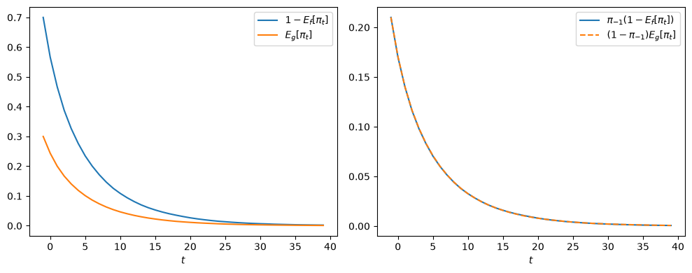
t =  0: (1 - E_f[π_t]) / E_g[π_t] = 2.325
t =  5: (1 - E_f[π_t]) / E_g[π_t] = 2.320
t = 10: (1 - E_f[π_t]) / E_g[π_t] = 2.335
t = 20: (1 - E_f[π_t]) / E_g[π_t] = 2.354
(1 - π_init) / π_init = 2.333
The two curves in the left panel differ by the factor \(7/3\); the two curves in the right panel coincide up to sampling error.
Part 3.
f = lambda w: p(w, 1, 1)
g = lambda w: p(w, 3, 1.2)
KL_fg = quad(lambda w: f(w) * np.log(f(w) / g(w)), 0, 1)[0]
KL_gf = quad(lambda w: g(w) * np.log(g(w) / f(w)), 0, 1)[0]

slope_F = np.polyfit(t_ex, np.median(lo_F, axis=0), 1)[0]
slope_G = np.polyfit(t_ex, np.median(lo_G, axis=0), 1)[0]
print(f"slope of median log odds under F: {slope_F:.3f},  KL(f, g) = {KL_fg:.3f}")
print(f"slope of median log odds under G: {slope_G:.3f}, -KL(g, f) = {-KL_gf:.3f}")
slope of median log odds under F: 0.754,  KL(f, g) = 0.759
slope of median log odds under G: -0.345, -KL(g, f) = -0.344
Typical paths converge faster under \(F\) than under \(G\).
Part 4.
We compute the Chernoff entropy and the minimizer \(s^*\).
A = lambda s: quad(lambda w: f(w)**s * g(w)**(1 - s), 0, 1)[0]
res = op.minimize_scalar(A, bounds=(0, 1), method='bounded')
s_star, C = res.x, -np.log(res.fun)
print(f"s* = {s_star:.3f}, C(f, g) = {C:.4f}")
s* = 0.597, C(f, g) = 0.1212
Next we estimate \(\log(1 - E_f[\pi_t])\) by importance sampling from \(m\) for \(t\) up to \(199\).
T_is, N_is = 200, 100_000
rng = np.random.default_rng(2025)
w = rng.beta(3 - 2 * s_star, 1.2 - 0.2 * s_star, size=(N_is, T_is))
log_L = np.cumsum(np.log(f(w)) - np.log(g(w)), axis=1)    # log L_t, t = 0, ..., 199
t_is = np.arange(T_is)

log_odds = np.log(π_init / (1 - π_init)) + log_L
weights = np.exp((1 - s_star) * log_L)                    # L_t^(1 - s*)
log_err_F = (t_is + 1) * np.log(A(s_star)) \
            + np.log(np.mean(expit(-log_odds) * weights, axis=0))

for t in [10, 20, 30]:
    print(f"t = {t}: log(1 - E_f[π_t]) importance sampling {log_err_F[t]:.3f}, "
          f"plain Monte Carlo {np.log(err_F[t+1]):.3f}")

late = t_is >= 100
slope = np.polyfit(t_is[late], log_err_F[late], 1)[0]
slope_adj = np.polyfit(t_is[late], log_err_F[late] + 0.5 * np.log(t_is[late] + 1), 1)[0]
print(f"slope of log(1 - E_f[π_t]) for t in [100, 199]: {slope:.4f}")
print(f"slope after adding log(t+1)/2:                 {slope_adj:.4f}")
print(f"-C(f, g):                                      {-C:.4f}")
t = 10: log(1 - E_f[π_t]) importance sampling -2.215, plain Monte Carlo -2.219
t = 20: log(1 - E_f[π_t]) importance sampling -3.638, plain Monte Carlo -3.626
t = 30: log(1 - E_f[π_t]) importance sampling -4.994, plain Monte Carlo -5.000
slope of log(1 - E_f[π_t]) for t in [100, 199]: -0.1243
slope after adding log(t+1)/2:                 -0.1209
-C(f, g):                                      -0.1212
The two estimates agree at small \(t\).
Under \(m\), \(E_m[\log \ell(w)] = A'(s^*)/A(s^*) = 0\), so \(\log L_t\) is a random walk without drift.
The expectation \(E_m[(1 - \pi_t) L_t^{1-s^*}]\) therefore decays only like \(t^{-1/2}\), and
for a constant \(K\).
The fitted slope is close to \(-C(f,g)\), and adding \(\frac{1}{2}\log(t+1)\) to remove the factor \(t^{-1/2}\) brings it closer.
By (28.8), \(E_g[\pi_t]\) decays at the same rate.
Exercise 28.3
A Pólya urn starts with \(a\) red balls and \(b\) black balls.
At each date \(t = 0, 1, \ldots\) we draw a ball at random, set \(W_t = 1\) if it is red and \(W_t = 0\) if it is black, and return it to the urn together with one more ball of the same color.
Show that \(\textrm{Prob}(W_0 = 1, W_1 = 0) = \textrm{Prob}(W_0 = 0, W_1 = 1)\). More generally, show that the probability of a sequence \((w_0, \ldots, w_{n-1})\) depends only on the number \(k\) of red draws, so that \(W_0, W_1, \ldots\) is exchangeable. Find the mixing measure \(\mu\) in de Finetti’s representation (28.3).
Simulate many urns with \(a = 2\) and \(b = 3\) for \(n = 2000\) draws. Compare the distribution across urns of the fraction of red draws with the Beta\((a, b)\) density.
Show that the fraction of red balls in the urn after \(n\) draws, \(k\) of them red, equals the probability \(\textrm{Prob}(W_n = 1 \,|\, w_0, \ldots, w_{n-1})\) that a Bayesian with a Beta\((a, b)\) prior over the success probability \(\theta\) of IID Bernoulli draws attaches to the next draw being red.
Solution
Part 1.
\(\textrm{Prob}(W_0 = 1, W_1 = 0) = \frac{a}{a+b} \frac{b}{a+b+1}\) and \(\textrm{Prob}(W_0 = 0, W_1 = 1) = \frac{b}{a+b} \frac{a}{a+b+1}\).
The two are equal.
For a sequence of \(n\) draws with \(k\) red draws, the denominators of the successive conditional probabilities are \(a+b, a+b+1, \ldots, a+b+n-1\) in every order.
The numerators for the red draws are \(a, a+1, \ldots, a+k-1\), and the numerators for the black draws are \(b, b+1, \ldots, b+n-k-1\), in every order.
So
where \(B\) is the Beta function.
The right side equals \(\int_0^1 \theta^k (1-\theta)^{n-k} \mu(d\theta)\) with \(\mu\) the Beta\((a,b)\) distribution.
That is de Finetti’s representation (28.3).
Part 2.
from scipy.stats import beta as beta_dist, kstest

def polya_urn(rng, a, b, n, N):
    "Simulate N Pólya urns for n draws; return the N x n array of draws."
    red = np.full(N, float(a))
    total = float(a + b)
    W = np.empty((N, n), dtype=np.int8)
    for t in range(n):
        W[:, t] = rng.random(N) < red / total
        red += W[:, t]
        total += 1
    return W

a, b, n, N = 2, 3, 2000, 20_000
rng = np.random.default_rng(7)
W = polya_urn(rng, a, b, n, N)
freq = W.mean(axis=1)

grid = np.linspace(0, 1, 200)
fig, ax = plt.subplots()
ax.hist(freq, bins=50, density=True, alpha=0.5,
        label=f'fraction of red draws, $n = {n}$')
ax.plot(grid, beta_dist.pdf(grid, a, b), lw=2, label=f'Beta$({a}, {b})$ density')
ax.set_xlabel(r'$\theta$')
ax.legend()
plt.show()

print(f"Prob(W_0=1, W_1=0) = {np.mean((W[:, 0] == 1) & (W[:, 1] == 0)):.4f}, "
      f"Prob(W_0=0, W_1=1) = {np.mean((W[:, 0] == 0) & (W[:, 1] == 1)):.4f}, "
      f"exact = {a * b / ((a + b) * (a + b + 1)):.4f}")
print(f"Kolmogorov-Smirnov test against Beta({a}, {b}): "
      f"p-value = {kstest(freq, beta_dist(a, b).cdf).pvalue:.3f}")
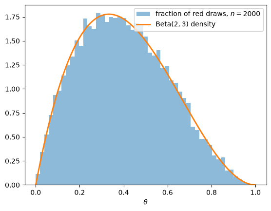
Prob(W_0=1, W_1=0) = 0.2033, Prob(W_0=0, W_1=1) = 0.2003, exact = 0.2000
Kolmogorov-Smirnov test against Beta(2, 3): p-value = 0.209
The fraction of red draws is distributed approximately Beta\((2, 3)\) across urns, and the Kolmogorov–Smirnov test does not reject that distribution.
Part 3.
After \(n\) draws with \(k\) red draws, the urn holds \(a + k\) red balls out of \(a + b + n\) balls, so the next draw is red with probability \((a+k)/(a+b+n)\).
A Bayesian with a Beta\((a, b)\) prior over \(\theta\) has the Beta\((a + k, b + n - k)\) posterior after observing \(k\) successes in \(n\) IID Bernoulli trials.
His probability that the next draw is a success is the posterior mean of \(\theta\), namely \((a + k)/(a + b + n)\).
The urn and the Bayesian agree.
The next cell checks this by grouping the simulated urns according to the number of red balls among the first \(10\) draws.
Frequencies computed from few urns are less precise.
n0 = 10
k = W[:, :n0].sum(axis=1)
for k_val in range(0, n0 + 1, 2):
    sel = k == k_val
    print(f"k = {k_val:2d} ({sel.sum():4d} urns): "
          f"frequency of red at draw {n0} = {W[sel, n0].mean():.3f}, "
          f"(a + k) / (a + b + n) = {(a + k_val) / (a + b + n0):.3f}")
k =  0 (1378 urns): frequency of red at draw 10 = 0.129, (a + k) / (a + b + n) = 0.133
k =  2 (2686 urns): frequency of red at draw 10 = 0.265, (a + k) / (a + b + n) = 0.267
k =  4 (2850 urns): frequency of red at draw 10 = 0.403, (a + k) / (a + b + n) = 0.400
k =  6 (2077 urns): frequency of red at draw 10 = 0.535, (a + k) / (a + b + n) = 0.533
k =  8 (1118 urns): frequency of red at draw 10 = 0.684, (a + k) / (a + b + n) = 0.667
k = 10 ( 218 urns): frequency of red at draw 10 = 0.839, (a + k) / (a + b + n) = 0.800