93. Exchange Rate Indeterminacy, Learning, and Experiments#
93.1. Overview#
In A Peculiar Definition of Bounded Rationality we met a model in which rational expectations cannot pin down the exchange rate at all.
Two fiat currencies, perfect substitutes as long as their rates of return are equal, leave the exchange rate \(e\) completely unrestricted: if the equilibrium conditions have a solution for one \(e\), they have a solution for every other, and the real allocation is identical across all of them.
This lecture, following Sargent [1993], expels the rational agents from that economy and puts adaptive ones in their place.
It is the hinge of the series.
Its first half uses the last of the series’ econometric learners, a Newton–Raphson rule like the one in Adaptive Agents in an Overlapping Generations Monetary Economy.
Its second half uses the series’ first genetic algorithm, a device that Networks, Genetic Algorithms, and Classifier Systems then sets out in general.
Two questions organize what follows.
First, does learning pin the exchange rate down?
An adaptive agent has beliefs, a rule for revising them, and initial conditions, and those initial conditions are exactly what the equilibrium conditions failed to determine.
We shall see that Newton–Raphson learners do converge to a constant exchange rate, but that learning does not select one.
Where they end up depends on where their portfolios and saving rates started, and also on how the learning algorithm is tuned.
Learning makes the exchange rate history-dependent: what Sargent calls the “dead hand of history” does the pinning that fundamentals refused to do.
Second, does a ghost of the indeterminacy survive?
It does.
The rest points of the learning algorithm reproduce the indeterminacy exactly: the condition that stops the algorithm is the same arbitrage condition that made the exchange rate free in the first place.
Sargent judges that an adaptive mechanism that selects the exchange rate path in this way “may seem a weak reed on which to base exchange rate determination.”
Then we turn to evidence.
Arifovic [1996] ran this economy as a laboratory experiment with paying human subjects.
Their exchange rate did not settle down.
When she replaced the Newton–Raphson learners with a genetic algorithm — a population of binary-string agents bred by selection, crossover, and mutation — she got an economy whose exchange rate does not settle down either.
The genetic population learns to save at close to the rational expectations rate, but nothing pins down its portfolio share, which wanders along the continuum of equilibria.
The ghost of indeterminacy returns as volatility.
That contrast — a learning rule that converges versus one that generates permanent volatility — is where this lecture lands.
Let’s start with some imports.
import numpy as np
import pandas as pd
import matplotlib.pyplot as plt
from typing import NamedTuple
93.2. The two-currency economy#
We use the overlapping generations incarnation of the Kareken and Wallace [1981] indeterminacy.
At each date \(t\), \(N\) two-period-lived agents are born, endowed with \(w_1\) when young and \(w_2\) when old, with \(w_1 > w_2\).
(As in Adaptive Agents in an Overlapping Generations Monetary Economy, the endowments are \(w_1\) and \(w_2\); A Peculiar Definition of Bounded Rationality writes them as \(2w_1\) and \(2w_2\).)
There are two fiat currencies in fixed supplies \(H_1\) and \(H_2\).
A young agent makes two decisions: how much to save, \(s_t\), and what fraction \(\lambda_t\) of that saving to hold in currency 1 (the rest going to currency 2).
The realized lifetime utility of an agent who chooses \((s_t, \lambda_t)\) is
where \(p_{it}\) is the price level in currency \(i\) and \(p_{it}/p_{i,t+1}\) is the gross return on holding currency \(i\).
We take \(u(c) = \ln c\) throughout.
Equating each currency’s supply to the demand for it gives the price levels
and the exchange rate is \(e_t = p_{1t}/p_{2t}\).
93.2.1. The indeterminacy, recalled#
Consider a stationary equilibrium with constant prices.
Then each currency returns \(p_{it}/p_{i,t+1} = 1\), so both returns are equal, and the portfolio return in (93.1) is \(1\) regardless of \(\lambda\).
The saving decision then solves \(\max_s \ln(w_1 - s) + \ln(w_2 + s)\), giving
but the portfolio share \(\lambda\) is completely undetermined: utility does not depend on it when the two returns are equal.
And \(\lambda\) is what fixes the exchange rate.
From (93.2), with a common \((s, \lambda)\),
Every \(\lambda \in (0, 1)\) is an equilibrium, so every \(e \in (0, \infty)\) is an equilibrium.
This is the indeterminacy of A Peculiar Definition of Bounded Rationality, now expressed through an undetermined portfolio choice.
This lecture runs two economies with different parameters.
The Newton–Raphson section uses Sargent’s \((w_1, w_2, H_1, H_2) = (20, 15, 100, 120)\), whose currency supplies are those of the two-currency example in A Peculiar Definition of Bounded Rationality.
The laboratory and genetic-algorithm sections use Arifovic’s \((11, 1, 10, 10)\).
So we carry the parameters in a container and pass them explicitly rather than leaving them lying about as globals.
class Params(NamedTuple):
    w1: float          # endowment when young
    w2: float          # endowment when old
    H1: float          # fixed supply of currency 1
    H2: float          # fixed supply of currency 2

    @property
    def s_star(self):
        "Rational expectations saving rate, when both currencies return 1."
        return (self.w1 - self.w2) / 2


kw = Params(w1=20.0, w2=15.0, H1=100.0, H2=120.0)

print(f"rational expectations saving rate s* = {kw.s_star}")
print(f"any portfolio share λ is an equilibrium, and e = (H1/H2)(1-λ)/λ is free")
rational expectations saving rate s* = 2.5
any portfolio share λ is an equilibrium, and e = (H1/H2)(1-λ)/λ is free
93.3. Newton–Raphson learning#
Now expel the rational agents.
As in Adaptive Agents in an Overlapping Generations Monetary Economy, a cohort’s lifetime utility cannot be evaluated until it is old, so the population is split into an “even” and an “odd” class.
Each class carries its own rule \((s, \lambda)\), updated only from the experience of earlier agents of the same class.
An agent revises \((s, \lambda)\) by a Newton–Raphson step against realized utility: move in the direction that a second-order expansion of (93.1) says would have raised utility, given the returns the agent actually experienced.
Writing \(\nabla U_\tau\) and \(\nabla^2 U_\tau\) for the gradient and Hessian of realized utility and \(M\) for a running estimate of the (negative-definite) Hessian, the recursion is
with \(\gamma_\tau\) a gain.
This is the two-variable version of the Robbins–Monro rule of Adaptive Agents in an Overlapping Generations Monetary Economy.
We use a constant gain, \(\gamma_\tau = \gamma = 0.3\), a variant that Sargent mentions in a footnote.
Because this economy has no shocks, a constant gain can still converge to a point.
Here are the gradient and Hessian of (93.1) in the returns \(R_1 = p_{1t}/p_{1,t+1}\) and \(R_2 = p_{2t}/p_{2,t+1}\).
def grad_hess(p, s, lam, R1, R2):
    "Gradient and Hessian of realized utility U(s, λ)."
    A = lam*R1 + (1 - lam)*R2               # portfolio gross return
    c2 = p.w2 + s*A                         # old-age consumption
    dR = R1 - R2
    g = np.array([-1/(p.w1 - s) + A/c2,
                  s*dR/c2])
    U_ss = -1/(p.w1 - s)**2 - A**2/c2**2
    U_ll = -s**2 * dR**2 / c2**2
    U_sl = dR/c2 - s*A*dR/c2**2
    return g, np.array([[U_ss, U_sl], [U_sl, U_ll]])
93.3.1. The indeterminacy shows up as a singular Hessian#
Look at the \(\lambda\) block of the Hessian.
When the two returns are equal, \(R_1 = R_2\), every \(\lambda\)-derivative vanishes: the gradient component \(s(R_1 - R_2)/c_2\) is zero, and so is the curvature \(-s^2(R_1 - R_2)^2/c_2^2\).
Utility is flat in \(\lambda\) at equal returns.
That is the indeterminacy, seen locally: there is no force pushing \(\lambda\) in any direction.
Near equal returns the curvature is of second order in \(R_1 - R_2\) while the gradient is of first order, so an undamped Newton step in \(\lambda\), which divides the gradient by the curvature, is enormous.
We therefore add a constant ridge \(\kappa > 0\) to the curvature estimate in the \(\lambda\) direction: each period we feed (93.3) the matrix \(\nabla^2 U_\tau - \mathrm{diag}(0, \kappa)\) in place of \(\nabla^2 U_\tau\).
This is a one-direction version of the Levenberg–Marquardt device of numerical optimization, and it is this lecture’s addition, not the book’s.
It is a stabilizer, not an enabler.
Without it the algorithm does not freeze; it explodes, as we check below.
With it, a \(\lambda\) step is roughly \(\gamma \, |\partial U/\partial \lambda| / \kappa\), so a large \(\kappa\) makes portfolios adjust sluggishly.
def newton_learning(p, s0, lam0, T=400, gain=0.3, κ=0.5, w2_path=None):
    """
    Two-currency OLG with Newton-Raphson learning of (s, λ), one rule per class
    (even/odd).  κ is a ridge added to the curvature estimate M in the
    λ direction.  w2_path optionally gives the old-age endowment at each date.
    """
    s = np.array(s0, float)
    lam = np.array(lam0, float)
    M = [np.array([[-1.0, 0.0], [0.0, -κ]]) for _ in range(2)]   # initial curvature
    p1 = np.empty(T)
    p2 = np.empty(T)
    e = np.empty(T)
    s_hist = np.empty((T, 2))
    lam_hist = np.empty((T, 2))

    for t in range(T):
        j = t % 2                                    # class that is young at t
        p1[t] = p.H1 / (lam[j]*s[j])
        p2[t] = p.H2 / ((1 - lam[j])*s[j])
        e[t] = p1[t] / p2[t]
        if t >= 1:                                   # class young at t-1 is now old
            jp = 1 - j
            R1, R2 = p1[t-1]/p1[t], p2[t-1]/p2[t]
            q = p if w2_path is None else p._replace(w2=w2_path[t])
            g, h = grad_hess(q, s[jp], lam[jp], R1, R2)
            h[1, 1] -= κ                             # the ridge
            M[jp] = M[jp] + gain*(h - M[jp])
            step = gain * np.linalg.solve(M[jp], g)
            s[jp] = np.clip(s[jp] - step[0], 0.1, p.w1 - 0.1)
            lam[jp] = np.clip(lam[jp] - step[1], 0.02, 0.98)
        s_hist[t] = s
        lam_hist[t] = lam

    return e, s_hist, lam_hist
93.3.2. Convergence to a history-dependent exchange rate#
Run two experiments that are identical except for the initial saving rates and portfolio shares.
e1, s1, l1 = newton_learning(kw, [3.5, 2.0], [0.35, 0.40])
e2, s2, l2 = newton_learning(kw, [2.0, 3.5], [0.62, 0.58])

fig, axes = plt.subplots(1, 3, figsize=(14, 4))

axes[0].plot(np.log(e1), 'C0', lw=1.3, label="experiment 1")
axes[0].plot(np.log(e2), 'C1', lw=1.3, label="experiment 2")
axes[0].set_title("log exchange rate")
axes[0].set_xlabel("$t$")
axes[0].legend(frameon=False)

for s_h, c in [(s1, 'C0'), (s2, 'C1')]:
    axes[1].plot(s_h[:, 0], color=c, lw=1.0)
    axes[1].plot(s_h[:, 1], color=c, lw=1.0, ls=':')
axes[1].axhline(kw.s_star, color='k', lw=0.8, ls='--')
axes[1].set_title("saving  (solid = even, dotted = odd)")
axes[1].set_xlabel("$t$")

for l_h, c in [(l1, 'C0'), (l2, 'C1')]:
    axes[2].plot(l_h[:, 0], color=c, lw=1.0)
    axes[2].plot(l_h[:, 1], color=c, lw=1.0, ls=':')
axes[2].set_title(r"portfolio share $\lambda$")
axes[2].set_xlabel("$t$")
plt.tight_layout()
plt.show()
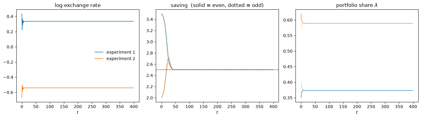
Fig. 93.1 Newton-Raphson learning from two initial conditions#
Both economies converge.
Saving climbs or falls to the rational expectations rate \(s^\star = 2.5\) from either side, and the two classes’ portfolio shares merge to a common value.
But the two experiments converge to different exchange rates.
for name, e, s_h, l_h in [("experiment 1", e1, s1, l1), ("experiment 2", e2, s2, l2)]:
    still = np.abs(np.diff(l_h, axis=0)).max(axis=1) > 1e-6
    t_freeze = np.flatnonzero(still)[-1] + 2         # λ moves by < 1e-6 from here on
    print(f"{name}: e → {e[-1]:.4f} (log e → {np.log(e[-1]):.3f}),  s → {s_h[-1][0]:.3f},  "
          f"λ → {l_h[-1][0]:.4f},  λ frozen from t = {t_freeze}")
experiment 1: e → 1.3998 (log e → 0.336),  s → 2.500,  λ → 0.3732,  λ frozen from t = 28
experiment 2: e → 0.5819 (log e → -0.541),  s → 2.500,  λ → 0.5888,  λ frozen from t = 35
The saving rate is pinned down by fundamentals; the exchange rate is pinned down by history.
Experiment 1’s limit is close to that of Sargent’s experiment 1, whose \(\lambda\) settles near \(0.37\) and whose log exchange rate settles near \(0.3\).
Sargent’s paths are still drifting after a few hundred periods, while with our constant gain \(\lambda\) stops moving within about \(35\) periods.
Before looking at how the limit depends on history, let’s check what the ridge \(\kappa\) does.
Here is experiment 1 again with \(\kappa = 0\).
e0, s0_h, l0_h = newton_learning(kw, [3.5, 2.0], [0.35, 0.40], κ=0.0)
print("last four exchange rates:", ", ".join(f"{x:.3f}" for x in e0[-4:]))
print(f"final λ (even, odd): {l0_h[-1]},  final s (even, odd): {s0_h[-1]}")
last four exchange rates: 40.833, 0.017, 40.833, 0.017
final λ (even, odd): [0.02 0.98],  final s (even, odd): [0.1 0.1]
Without the ridge the algorithm does not stand still.
The curvature estimate stays invertible, but its \(\lambda\) entry is tiny, so the \(\lambda\) steps are huge.
The portfolio shares crash into the bounds \(0.02\) and \(0.98\) that the code imposes, saving collapses to its lower bound, and from then on the exchange rate flips between two extreme values.
93.3.3. The dead hand of history#
To see how history governs the outcome, sweep the initial portfolio shares and record the exchange rate each economy settles on.
The two classes must start with different portfolio shares.
If they start with the same \(\lambda_0\), the exchange rate, which depends only on the young class’s \(\lambda\), is constant from the first period on.
Then \(R_1 = R_2\) from the start, the \(\lambda\)-gradient is identically zero, and \(\lambda\) never moves, so the limit would be \((H_1/H_2)(1-\lambda_0)/\lambda_0\) by construction.
So we start the even and odd classes at \(\bar\lambda_0 - 0.05\) and \(\bar\lambda_0 + 0.05\), with experiment 1’s saving rates, and plot each limit against the mean initial share \(\bar\lambda_0\).
We compare the limits with the curve \((H_1/H_2)(1-\lambda)/\lambda\) evaluated at two points: the limiting share \(\lambda_\infty\), and the mean initial share \(\bar\lambda_0\).
def e_of_λ(p, lam):
    "Exchange rate when every agent holds portfolio share λ."
    return (p.H1/p.H2) * (1 - lam) / lam


λ_bar0 = np.linspace(0.15, 0.85, 15)
e_lim = np.empty_like(λ_bar0)
λ_lim = np.empty_like(λ_bar0)
for k, lb in enumerate(λ_bar0):
    e, s_h, l_h = newton_learning(kw, [3.5, 2.0], [lb - 0.05, lb + 0.05])
    e_lim[k], λ_lim[k] = e[-1], l_h[-1].mean()

fig, ax = plt.subplots(figsize=(7, 4.5))
ax.plot(λ_bar0, e_lim, 'C0o', ms=6, label="limiting $e$ from learning")
ax.plot(λ_bar0, e_of_λ(kw, λ_lim), 'C0-', lw=1,
        label=r"$(H_1/H_2)(1-\lambda_\infty)/\lambda_\infty$")
ax.plot(λ_bar0, e_of_λ(kw, λ_bar0), 'k--', lw=1,
        label=r"$(H_1/H_2)(1-\bar\lambda_0)/\bar\lambda_0$")
ax.set_yscale('log')
ax.set_xlabel(r"mean initial portfolio share $\bar\lambda_0$")
ax.set_ylabel("limiting exchange rate $e$")
ax.legend(frameon=False)
plt.show()
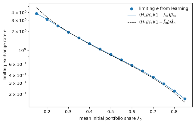
Fig. 93.2 Limiting exchange rate against the mean initial portfolio share#
Here are the gaps between the limits and the two curves.
gap_lim = np.abs(e_lim / e_of_λ(kw, λ_lim) - 1)
gap_init = np.abs(e_lim / e_of_λ(kw, λ_bar0) - 1)
print(f"largest relative gap from the curve at λ∞:  {gap_lim.max():.1e}")
print(f"relative gap from the curve at mean λ0:     "
      f"{gap_init.min():.3f} to {gap_init.max():.3f}")
largest relative gap from the curve at λ∞:  2.2e-16
relative gap from the curve at mean λ0:     0.005 to 0.191
Every limit lies exactly on the rational expectations continuum, evaluated at its own limiting \(\lambda\): each one is an equilibrium.
The zero gap is close to automatic: in every period, transients included, the exchange rate is \((H_1/H_2)(1-\lambda)/\lambda\) at the young class’s share, so all the gap confirms is that the two classes’ shares have merged.
The informative comparison is with the dashed curve.
As \(\bar\lambda_0\) sweeps from \(0.15\) to \(0.85\), the limits trace out a wide stretch of the continuum.
But the limit is not simply the equilibrium that the mean initial share implies.
While the two classes still differ, the two currencies’ returns differ, and those transient return gaps push \(\lambda\) around before the arbitrage condition shuts the motion off.
The gaps from the dashed curve range from half a percent to almost twenty percent.
They are largest at the edges of the grid, where the classes’ initial shares imply very different exchange rates.
This is what Sargent means by the dead hand of history:
Our learning system renders the exchange rate path determinate by having the ‘dead hand of history’ put enough sluggishness into decisions. The exchange rate path can be said to be ‘history-dependent’ because the initial conditions assigned to \((\lambda, s)\) assume an importance that does not vanish as time passes.
The relevant history is more than the initial portfolio shares.
The limit also depends on the initial saving rates and on the tuning of the algorithm, the ridge \(\kappa\) and the gain \(\gamma\); Exercise 93.1 measures both.
Learning converts an indeterminacy of levels into a dependence on history.
It makes the exchange rate history-dependent; it does not select one.
93.3.4. The ghost of indeterminacy#
Why does the exchange rate freeze rather than move to some particular value?
Because the algorithm comes to rest wherever the gradient vanishes, and the portfolio gradient \(s(R_1 - R_2)/c_2\) vanishes precisely when \(R_1 = R_2\), the arbitrage condition that made the exchange rate free under rational expectations.
Let’s compute the returns and the gradient at the end of experiment 1, and the \(\lambda\) derivatives at other points of the continuum.
s_lim, lam_lim = s1[-1], l1[-1]                  # (even, odd) rules at the end
p1_lim = kw.H1 / (lam_lim*s_lim)                 # price levels when each class is young
p2_lim = kw.H2 / ((1 - lam_lim)*s_lim)
R1, R2 = p1_lim[1]/p1_lim[0], p2_lim[1]/p2_lim[0]  # returns to an odd agent
g, h = grad_hess(kw, s_lim[1], lam_lim[1], R1, R2)
print(f"end of experiment 1: R1 = {R1:.6f}, R2 = {R2:.6f}, gradient = {g.round(8) + 0.0}")

print("\nλ derivatives at other rest points (s = s*, R1 = R2 = 1):")
for lam in (0.2, 0.5, 0.8):
    g, h = grad_hess(kw, kw.s_star, lam, 1.0, 1.0)
    print(f"  λ = {lam}:  ∂U/∂λ = {g[1] + 0.0:.1f},  ∂²U/∂λ² = {h[1, 1] + 0.0:.1f},  "
          f"e = {e_of_λ(kw, lam):.3f}")
end of experiment 1: R1 = 1.000000, R2 = 1.000000, gradient = [0. 0.]

λ derivatives at other rest points (s = s*, R1 = R2 = 1):
  λ = 0.2:  ∂U/∂λ = 0.0,  ∂²U/∂λ² = 0.0,  e = 3.333
  λ = 0.5:  ∂U/∂λ = 0.0,  ∂²U/∂λ² = 0.0,  e = 0.833
  λ = 0.8:  ∂U/∂λ = 0.0,  ∂²U/∂λ² = 0.0,  e = 0.208
The rest points of the learning dynamics are the rational expectations equilibria, exchange rate and all: a whole continuum of them.
One recursion, many learners explains how the limit of a learning recursion is governed by its linearization near a rest point: a rest point attracts when the linearized algorithm contracts in every direction.
A continuum of rest points rules that out in one direction, and shows up as an eigenvalue of exactly one.
Shift both classes’ portfolio shares by the same amount and nothing pulls them back, because the shifted point is another rest point.
To see this, compute the Jacobian of two periods of the algorithm (one update of each class) at experiment 1’s limit, by finite differences.
We hold the curvature estimate \(M\) at its limit, which loses nothing to first order, because the Newton step multiplies \(M^{-1}\) by a gradient that vanishes at the rest point.
def two_period_map(p, z, M, gain=0.3):
    "One update of each class's (s, λ), with the curvature estimate held at M."
    s, lam = z[:2].copy(), z[2:].copy()
    for jp in (1, 0):                                # the odd class updates, then the even
        j = 1 - jp
        R1 = lam[j]*s[j] / (lam[jp]*s[jp])           # p1 when jp was young / p1 now
        R2 = (1 - lam[j])*s[j] / ((1 - lam[jp])*s[jp])
        g, _ = grad_hess(p, s[jp], lam[jp], R1, R2)
        step = gain * np.linalg.solve(M, g)
        s[jp], lam[jp] = s[jp] - step[0], lam[jp] - step[1]
    return np.concatenate([s, lam])


def rest_point_jacobian(p, lam, κ=0.5, gain=0.3, ε=1e-6):
    "Jacobian of the two-period map at the rest point (s*, s*, λ, λ)."
    z = np.array([p.s_star, p.s_star, lam, lam])
    _, M = grad_hess(p, p.s_star, lam, 1.0, 1.0)     # Hessian at the rest point,
    M[1, 1] -= κ                                     # plus the ridge: the limit of M
    return np.column_stack([(two_period_map(p, z + ε*d, M, gain)
                             - two_period_map(p, z - ε*d, M, gain)) / (2*ε)
                            for d in np.eye(4)])


J = rest_point_jacobian(kw, lam_lim[0])
eigvals, eigvecs = np.linalg.eig(J)
order = np.argsort(-np.abs(eigvals))
labels = ["s even", "s odd", "λ even", "λ odd"]
print(pd.DataFrame(eigvecs[:, order].real, index=labels,
                   columns=[f"{v:.4f}" for v in eigvals[order].real]).round(3))
        1.0000  0.4014  0.2500  0.1600
s even   0.000   0.000   0.447   0.371
s odd    0.000   0.000   0.894   0.928
λ even   0.707  -0.535   0.000   0.000
λ odd    0.707   0.845   0.000   0.000
The columns are the eigenvectors, headed by their eigenvalues.
The eigenvalue of one belongs to the direction that moves both classes’ \(\lambda\) together: the continuum.
The next eigenvalue belongs to a direction that moves the two classes’ portfolio shares in opposite directions, and the two smallest belong to saving.
All three are below one, so saving returns to \(s^\star\) and the classes’ shares merge.
But the place on the continuum where they merge is whatever the stable directions left behind.
That is the dead hand of history, written as an eigenvalue.
The indeterminacy is not resolved; it is displaced into the initial conditions and the tuning of the algorithm.
Sargent’s verdict is hedged but clear.
By tying down the expectations that the rational expectations equilibrium left free, he writes, the adaptive mechanism selects an exchange rate path, but
This may seem a weak reed on which to base exchange rate determination.
A footnote adds:
Put differently, a regime that allows the exchange rate to be history-dependent seems to be an ill-formed mechanism.
The ghost stays quiet here only because the Newton–Raphson learner stops experimenting once the returns are equal.
A learning rule that keeps experimenting can wake it, as the evidence below shows.
93.4. Evidence from the laboratory#
Arifovic [1996] implemented this two-currency economy as an experiment with paying human subjects, using \(w_1 = 11\), \(w_2 = 1\), \(H_1 = H_2 = 10\), so that \(s^\star = 5\).
These are not the parameters of the Newton–Raphson section above; Exercise 93.4 runs the Newton–Raphson learner at Arifovic’s parameters.
Each young subject chose a saving rate and a fraction to allocate between the two currencies; the experimenters cleared the two money markets against those choices, exactly as in (93.2).
Arifovic split her subjects into two groups of equal size, one young in odd periods and the other in even periods.
These alternating groups are the laboratory counterpart of the odd and even classes of our learners.
The experiment ended in a period that the subjects did not know in advance.
The money held by that last young generation was redeemed at the average of the previous two periods’ price levels.
The result did not look like the Newton–Raphson simulations at all.
The exchange rate fluctuated persistently, roughly within a band from \(0.5\) to \(2\), and showed no sign of settling down.
If anything the amplitude grew between the second and third sessions.
The simple Newton–Raphson model, which at Sargent’s parameters converges to a constant, does a poor job of matching that.
So Arifovic built a different model of the same economy, one in which the agents are a population bred by a genetic algorithm.
93.5. A genetic algorithm economy#
Networks, Genetic Algorithms, and Classifier Systems sets out Holland’s genetic algorithm in general; here we need only the version Arifovic used.
Now each class is a population of \(N = 30\) agents, and each agent is a binary string of length \(30\): the first \(20\) bits encode its saving rate, the last \(10\) its portfolio share.
Every period the young population’s strings are decoded into \((s_i, \lambda_i)\) pairs, the two money markets clear against the aggregates via (93.2), and the exchange rate is read off.
A generation later, when the cohort is old, each string’s realized utility (93.1) is its fitness, and the genetic algorithm breeds the next generation.
N, L_s, L_lam = 30, 20, 10           # population size; bits for saving and portfolio

arifovic = Params(w1=11.0, w2=1.0, H1=10.0, H2=10.0)

def decode(p, pop):
    "Binary strings → (s, λ), with s in (0, w1) and λ in [0.02, 0.98]."
    ints_s = pop[:, :L_s] @ (1 << np.arange(L_s)[::-1])
    ints_l = pop[:, L_s:] @ (1 << np.arange(L_lam)[::-1])
    s = 0.05 + (p.w1 - 0.10) * ints_s / (2**L_s - 1)
    lam = 0.02 + 0.96 * ints_l / (2**L_lam - 1)
    return s, lam

def fitness(p, pop, R1, R2):
    "Realized lifetime utility of each string given the returns it experienced."
    s, lam = decode(p, pop)
    c2 = p.w2 + s*(lam*R1 + (1 - lam)*R2)
    return np.log(p.w1 - s) + np.log(np.maximum(c2, 1e-9))
The genetic algorithm has the classic three operators — roulette-wheel selection of parents, single-point crossover, and bit-flip mutation — plus one that Arifovic introduced, the election operator: a child is admitted to the next generation only if it would have been fitter than its parent on the most recent returns, otherwise the parent survives.
Some details of our implementation are this lecture’s own choices, not necessarily Arifovic’s:
a mutation probability of \(0.033\) per bit;
crossover applied to every pair of parents;
a roulette wheel whose weights are fitness minus the population’s minimum fitness (a “windowed” wheel, needed because log utility can be negative);
the decoding ranges for \(s\) and \(\lambda\).
def genetic_step(p, pop, R1, R2, rng, p_mut=0.033, election=True):
    "Breed one new generation from the current one."
    fit = fitness(p, pop, R1, R2)
    weight = fit - fit.min() + 1e-6                  # windowed roulette wheel
    new = np.empty_like(pop)
    for k in range(0, N, 2):
        i, j = np.searchsorted(np.cumsum(weight), rng.random(2) * weight.sum())
        parents = np.array([pop[i], pop[j]])
        cut = rng.integers(1, L_s + L_lam)           # single-point crossover
        kids = parents.copy()
        kids[0, cut:], kids[1, cut:] = parents[1, cut:], parents[0, cut:]
        for c in kids:                               # mutation
            c[rng.random(L_s + L_lam) < p_mut] ^= 1
        if election:                                 # Arifovic's election operator
            f_kids = fitness(p, kids, R1, R2)
            f_par = fitness(p, parents, R1, R2)
            for m in range(2):
                new[k + m] = kids[m] if f_kids[m] > f_par[m] else parents[m]
        else:
            new[k], new[k + 1] = kids
    return new


def genetic_economy(p, T=3000, seed=0, election=True):
    """
    Run the genetic-algorithm economy.  Returns the exchange rate e_t and, for
    the population that is young at t, the mean and standard deviation of s
    and of λ across its strings.
    """
    rng = np.random.default_rng(seed)
    pops = [rng.integers(0, 2, (N, L_s + L_lam)) for _ in range(2)]   # even, odd
    p1 = np.empty(T)
    p2 = np.empty(T)
    stats = np.empty((T, 4))                         # mean s, sd s, mean λ, sd λ
    for t in range(T):
        j = t % 2
        s, lam = decode(p, pops[j])
        p1[t], p2[t] = p.H1 / np.sum(lam*s), p.H2 / np.sum((1 - lam)*s)
        stats[t] = s.mean(), s.std(), lam.mean(), lam.std()
        if t >= 1:
            jp = 1 - j
            R1, R2 = p1[t-1]/p1[t], p2[t-1]/p2[t]
            pops[jp] = genetic_step(p, pops[jp], R1, R2, rng, election=election)
    return p1 / p2, stats
93.5.1. Volatility that does not die out#
Let’s run the economy for \(4000\) periods and drop the first \(500\) as a burn-in.
Because every string’s \(\lambda\) lies in \([0.02, 0.98]\) and \(H_1 = H_2\), the exchange rate is confined to \([1/49, 49]\), so \(|\log e_t| \leq \ln 49 \approx 3.89\).
The dotted lines in the figure mark those bounds, and the shaded band marks the experimental range \([0.5, 2]\).
burn = 500
e_ga, stats_ga = genetic_economy(arifovic, T=4000, seed=1)
t_ga = np.arange(burn, len(e_ga))
log_e = np.log(e_ga[burn:])
bound = np.log(0.98 / 0.02)

fig, ax = plt.subplots(figsize=(10, 4))
ax.plot(t_ga, log_e, lw=0.5)
ax.axhspan(np.log(0.5), np.log(2), color='C1', alpha=0.2, label="experimental range")
for b in (bound, -bound):
    ax.axhline(b, color='k', ls=':', lw=0.8)
ax.set_xlabel("$t$")
ax.set_ylabel(r"$\log e_t$")
ax.legend(frameon=False, loc='upper right')
plt.show()
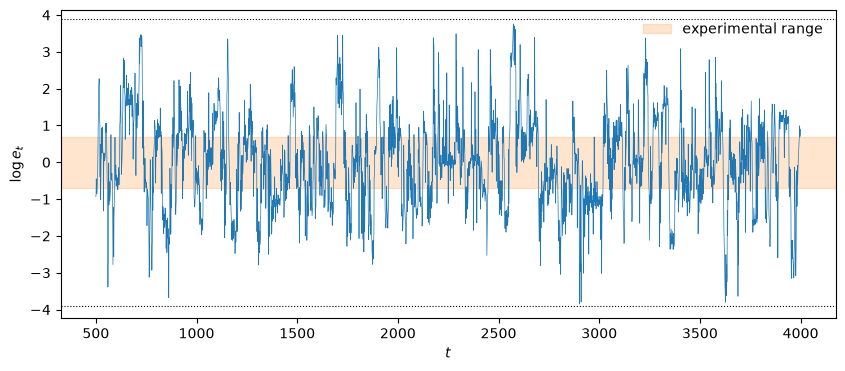
Fig. 93.3 Exchange rate in the genetic-algorithm economy#
The exchange rate wanders and keeps wandering, and it does so far outside the experimental range.
in_band = np.mean((e_ga[burn:] > 0.5) & (e_ga[burn:] < 2))
print(f"e ranges from {e_ga[burn:].min():.3f} to {e_ga[burn:].max():.1f}; "
      f"share of periods in [0.5, 2]: {in_band:.2f}")
print(f"largest |log e| = {np.abs(log_e).max():.2f}, against the bound {bound:.2f}")
print(f"standard deviation of log e, t = 500-1499: {np.log(e_ga[500:1500]).std():.3f}")
print(f"standard deviation of log e, t = 3000-3999: {np.log(e_ga[3000:]).std():.3f}")
e ranges from 0.021 to 42.8; share of periods in [0.5, 2]: 0.43
largest |log e| = 3.85, against the bound 3.89
standard deviation of log e, t = 500-1499: 1.279
standard deviation of log e, t = 3000-3999: 1.194
The volatility is a permanent feature, not a transient: it is about as large late in the run as early.
It is also bigger than in the laboratory.
Fewer than half the periods fall inside the experimental band, and the series comes close to the bounds that the encoding imposes.
Sargent noted the same thing about Arifovic’s genetic economy, whose exchange rates were “more variable than those found in Arifovic’s experiments.”
93.5.2. What the population learns#
Unlike the Newton–Raphson learner, the genetic population never settles down completely, since mutation keeps injecting new strings.
But it does learn, and what it learns and what it cannot learn line up with the stable and the neutral directions of The ghost of indeterminacy.
To see this, look at the young population’s mean and spread of \(s\) and of \(\lambda\) over a stretch of the run.
window = np.arange(2000, 2300)
fig, axes = plt.subplots(2, 1, figsize=(10, 6), sharex=True)
for ax, (m, sd), name in zip(axes, [(0, 1), (2, 3)], ["saving $s$", r"portfolio share $\lambda$"]):
    mean, spread = stats_ga[window, m], stats_ga[window, sd]
    ax.plot(window, mean, lw=1, label="population mean")
    ax.fill_between(window, mean - spread, mean + spread, alpha=0.3,
                    label="± within-population s.d.")
    ax.set_ylabel(name)
axes[0].axhline(arifovic.s_star, color='k', ls='--', lw=0.8, label="$s^\\star$")
axes[0].legend(frameon=False, ncol=3, loc='upper right')
axes[1].set_ylim(0, 1)
axes[1].set_xlabel("$t$")
plt.tight_layout()
plt.show()
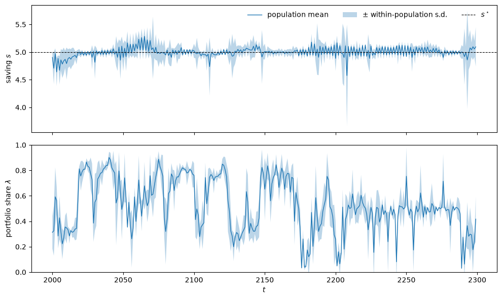
Fig. 93.4 Saving and portfolio shares inside the genetic population#
Here are the same statistics averaged over the whole run after the burn-in.
S = stats_ga[burn:]
print(f"mean saving: {S[:, 0].mean():.3f}   (s* = {arifovic.s_star})")
print(f"within-population s.d. of s: {S[:, 1].mean():.3f}")
print(f"within-population s.d. of λ: {S[:, 3].mean():.3f}")
print(f"s.d. over time of the population's mean λ: {S[:, 2].std():.3f}  "
      f"(a uniform draw on [0.02, 0.98] has s.d. {0.96/np.sqrt(12):.3f})")
print(f"5th and 95th percentiles of the population's mean λ: "
      f"{np.percentile(S[:, 2], 5):.2f}, {np.percentile(S[:, 2], 95):.2f}")
mean saving: 4.990   (s* = 5.0)
within-population s.d. of s: 0.110
within-population s.d. of λ: 0.092
s.d. over time of the population's mean λ: 0.237  (a uniform draw on [0.02, 0.98] has s.d. 0.277)
5th and 95th percentiles of the population's mean λ: 0.11, 0.88
The genetic economy settles in one direction and drifts in the other.
In the determinate direction, saving, the population learns: mean saving sits at \(s^\star\) and the strings agree closely with one another.
The strings also agree fairly closely about \(\lambda\) at any moment.
But the population’s common \(\lambda\) wanders over most of the range the encoding allows, and the exchange rate wanders with it.
The reason is the ghost of indeterminacy.
Nothing in the fundamentals favors one portfolio share over another: at equal returns every share is equally fit.
A share becomes fitter than another only when the two currencies’ returns differ, and they differ only because one cohort’s portfolio differs from the previous cohort’s.
So fitness is neutral in \(\lambda\) apart from return gaps that the population creates itself, and nothing anchors the population’s portfolio.
Mutation, crossover, and those self-generated return gaps push it along the continuum of equilibria, and nothing holds it in place.
The indeterminacy that the Newton–Raphson learner froze into a history-dependent constant returns here as volatility.
The election operator does much of the population’s learning; Exercise 93.2 shows what happens without it.
93.5.3. The shape of the volatility#
Sargent describes the exchange rate in Arifovic’s genetic economy as close to a random walk — but with mean reversion, showing up as a dip at zero frequency in the spectrum of its first difference.
We plot the spectrum of the winsorized \(\Delta \log e_t\) against frequency in radians on a log scale, as Sargent does, together with the autocorrelation of \(\log e_t\).
def averaged_spectrum(x, n_seg=16):
    "Bartlett-averaged periodogram; frequencies in radians per period."
    x = x - x.mean()
    seg = len(x) // n_seg
    acc = np.zeros(seg // 2 + 1)
    for k in range(n_seg):
        acc += np.abs(np.fft.rfft(x[k*seg:(k+1)*seg]))**2 / seg
    return 2 * np.pi * np.fft.rfftfreq(seg), acc / n_seg


d_log_e = np.diff(log_e)
d_log_e = np.clip(d_log_e, *np.percentile(d_log_e, [1, 99]))    # winsorize tails
freq, spec = averaged_spectrum(d_log_e)

def acf(x, K):
    x = x - x.mean()
    return np.array([np.sum(x[k:]*x[:len(x)-k]) / np.sum(x*x) for k in range(K)])


fig, axes = plt.subplots(1, 2, figsize=(12, 4))
axes[0].semilogy(freq[1:], spec[1:], lw=1.2)
axes[0].set_title(r"spectrum of $\Delta \log e$")
axes[0].set_xlabel("frequency (radians)")

axes[1].bar(range(25), acf(log_e, 25))
axes[1].set_title(r"autocorrelation of $\log e$")
axes[1].set_xlabel("lag")
plt.tight_layout()
plt.show()
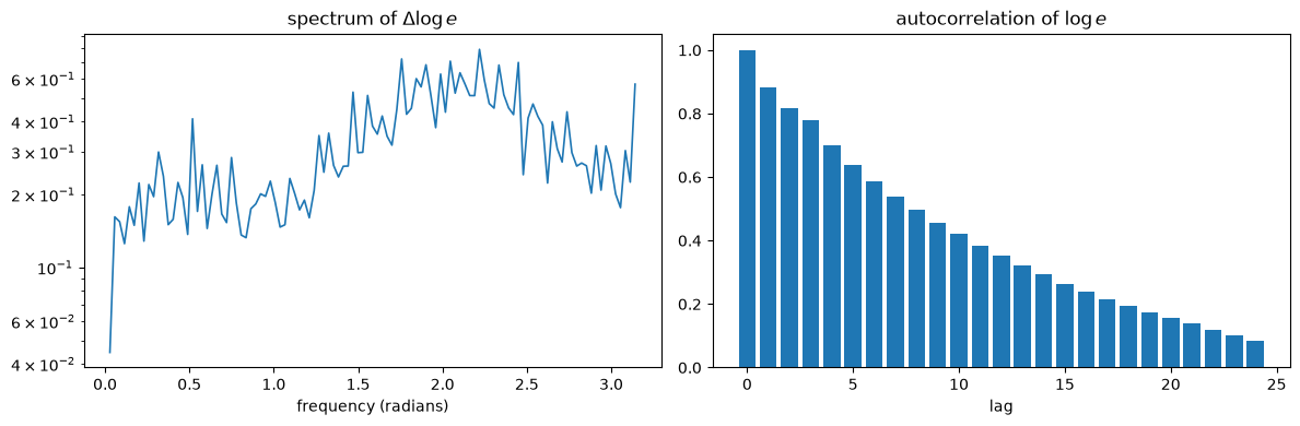
Fig. 93.5 Spectrum and autocorrelation of the exchange rate#
The spectrum is hump-shaped.
It is low near zero frequency, rises to a peak at intermediate frequencies, and falls off toward \(\pi\), much like the spectrum in Sargent’s figure, which peaks near \(1.5\) radians.
The autocorrelation of the level falls to one half by about lag \(8\) and is close to zero by lag \(25\).
That is much faster than a near unit root would allow.
But the sample autocorrelation is only an informal guide, because a random walk’s sample autocorrelation also decays in a finite sample.
A direct test is to regress \(\log e_t\) on a constant and \(\log e_{t-1}\) and compare the coefficient \(\hat\phi\) with one.
The Dickey–Fuller statistic \((\hat\phi - 1)/\mathrm{se}(\hat\phi)\) rejects a unit root at the 5% level when it is below about \(-2.86\).
def ar1(x):
    "OLS of x_t on (1, x_{t-1}): returns φ̂ and the Dickey-Fuller statistic."
    X = np.column_stack([np.ones(len(x) - 1), x[:-1]])
    b = np.linalg.lstsq(X, x[1:], rcond=None)[0]
    u = x[1:] - X @ b
    se = np.sqrt(u @ u / (len(u) - 2) * np.linalg.inv(X.T @ X)[1, 1])
    return b[1], (b[1] - 1) / se


band = slice(1, len(spec)//2)
φ, df_stat = ar1(log_e)
print(f"spectrum of Δlog e at the lowest frequency / mean over (0, π/2): "
      f"{spec[1] / spec[band].mean():.2f}")
print(f"spectral peak at frequency {freq[1:][np.argmax(spec[1:])]:.2f} radians")
print(f"AR(1) coefficient φ = {φ:.3f},  half-life = {np.log(0.5)/np.log(φ):.1f} periods")
print(f"Dickey-Fuller statistic = {df_stat:.1f}   (5% critical value ≈ -2.86)")
spectrum of Δlog e at the lowest frequency / mean over (0, π/2): 0.21
spectral peak at frequency 2.22 radians
AR(1) coefficient φ = 0.882,  half-life = 5.5 periods
Dickey-Fuller statistic = -14.8   (5% critical value ≈ -2.86)
The dip at zero frequency is pronounced.
The spectrum peaks near \(2.2\) radians, a cycle of about three periods.
The level is strongly mean-reverting, with a half-life of about five and a half periods, and the Dickey–Fuller test rejects a unit root decisively; Exercise 93.3 checks other seeds.
So in our implementation the genetic exchange rate is a stationary series, not a near random walk.
Part of the mean reversion is mechanical: the encoding’s bounds on \(\lambda\) cap \(|\log e_t|\), so the series cannot wander off for good.
Sargent’s assessment is that real floating exchange rates for hard-currency pairs have spectra of log differences that look much like Arifovic’s, except without the dip at zero frequency.
Actual exchange rates are even closer to pure random walks: it is hard to find a model that forecasts them better than “no change,” a benchmark that the neural-network forecasts of Kuan and Liu [1995] set out to beat.
So the genetic economy matches the higher-frequency texture of floating rates but not their lowest frequencies.
That it gets that far with no fundamental shocks at all, from a population of adapting agents repricing two intrinsically identical currencies, is the striking part.
93.6. Concluding remarks#
Two models of the same indeterminate economy gave two very different verdicts.
The Newton–Raphson learner converges — and in converging, exposes the indeterminacy rather than curing it.
Its rest points satisfy the arbitrage condition that leaves the exchange rate free.
They form a continuum, along which the algorithm has a unit eigenvalue.
So the limit is wherever the transient leaves the economy, and it depends on the initial portfolios and saving rates and on the tuning of the algorithm.
Learning makes the exchange rate history-dependent; it does not select one on any economic ground.
Sargent’s hedged verdict is that such a mechanism “may seem a weak reed.”
The genetic-algorithm economy does not converge, but not because it fails to learn.
With Arifovic’s election operator, the population learns a saving rate close to \(s^\star\) and becomes nearly homogeneous.
What it cannot learn is a portfolio share, because at equal returns no share is fitter than any other.
So the population’s common \(\lambda\) wanders along the continuum of equilibria, and the exchange rate wanders with it.
The ghost of indeterminacy returns as volatility, in an economy with no fundamental disturbances whatsoever.
That volatility is an instance of one of the payoffs that What the program is good for lists for the bounded-rationality program: a new source of dynamics.
It resembles the higher-frequency texture of floating exchange rates but not their low frequencies, where the genetic economy’s strong mean reversion has no counterpart in the data.
The two halves of the lecture also use different calibrations.
Exercise 93.4 runs the Newton–Raphson learner at Arifovic’s, and finds that it converges there only if it is damped enough.
With this lecture’s damping it sits on the edge of stability, and it generates recurrent bursts of volatility of its own.
Which learning model an economist reaches for, and how she tunes it, is one more of the choices that the bounded-rationality program forces into the open.
Networks, Genetic Algorithms, and Classifier Systems sets out Holland’s genetic algorithm in general, together with its richer cousin, the classifier system.
Money as a Medium of Exchange among Artificially Intelligent Agents then puts populations of classifier systems to work: they must not merely tune a portfolio but discover from scratch which good will serve as money.
93.7. Exercises#
Exercise 93.1
The main text varied the initial portfolio shares.
This exercise asks whether anything else matters for the limit.
Hold the initial portfolio shares fixed at \(\lambda_0 = (0.30, 0.50)\) for the (even, odd) classes, and vary the initial saving rates \(s_0\) over a few values. Confirm that the classes’ shares merge and saving converges to \(s^\star\). Does the limiting exchange rate change with \(s_0\)?
Start from experiment 1’s initial condition and vary the ridge \(\kappa\) over \((0.1, 0.2, 0.5, 1, 2)\), holding \(\gamma = 0.3\). Then vary the gain \(\gamma\) over \((0.05, 0.1, 0.3)\), holding \(\kappa = 0.5\). Record the limiting exchange rate each time.
Is the limiting exchange rate a function of the initial portfolio shares alone?
Solution
Here is part 1.
rows = []
for s0 in ([3.0, 2.2], [2.2, 3.0], [4.0, 4.0], [1.0, 1.0], [6.0, 2.0]):
    e, s_h, l_h = newton_learning(kw, s0, [0.30, 0.50], T=800)
    rows.append([str(s0), l_h[-1][0], l_h[-1][1], s_h[-1].mean(), e[-1]])

pd.DataFrame(rows, columns=["initial s", "λ even (limit)", "λ odd (limit)",
                            "s (limit)", "e (limit)"]).round(4)
| initial s | λ even (limit) | λ odd (limit) | s (limit) | e (limit) | |
|---|---|---|---|---|---|
| 0 | [3.0, 2.2] | 0.4117 | 0.4117 | 2.5 | 1.1908 |
| 1 | [2.2, 3.0] | 0.4471 | 0.4471 | 2.5 | 1.0304 |
| 2 | [4.0, 4.0] | 0.4444 | 0.4444 | 2.5 | 1.0418 |
| 3 | [1.0, 1.0] | 0.4145 | 0.4145 | 2.5 | 1.1773 |
| 4 | [6.0, 2.0] | 0.3772 | 0.3772 | 2.5 | 1.3759 |
The two classes’ shares merge (columns 2 and 3 agree), and saving converges to \(s^\star = 2.5\).
But the limiting exchange rate changes with the initial saving rates, even though the initial portfolio shares are the same in every row.
The \(\lambda\)-gradient \(s(R_1 - R_2)/c_2\) is proportional to saving, and the returns during the transient depend on both classes’ saving.
So saving’s path to \(s^\star\) shapes how far \(\lambda\) moves before the arbitrage condition stops it.
Here is part 2.
rows = []
for κ in (0.1, 0.2, 0.5, 1.0, 2.0):
    e, s_h, l_h = newton_learning(kw, [3.5, 2.0], [0.35, 0.40], T=2000, κ=κ)
    rows.append([κ, 0.3, l_h[-1][0], e[-1]])
for gain in (0.05, 0.1, 0.3):
    e, s_h, l_h = newton_learning(kw, [3.5, 2.0], [0.35, 0.40], T=4000, gain=gain)
    rows.append([0.5, gain, l_h[-1][0], e[-1]])

pd.DataFrame(rows, columns=["κ", "gain γ", "λ (limit)", "e (limit)"]).round(4)
| κ | gain γ | λ (limit) | e (limit) | |
|---|---|---|---|---|
| 0 | 0.1 | 0.30 | 0.5445 | 0.6970 |
| 1 | 0.2 | 0.30 | 0.3859 | 1.3263 |
| 2 | 0.5 | 0.30 | 0.3732 | 1.3998 |
| 3 | 1.0 | 0.30 | 0.3709 | 1.4136 |
| 4 | 2.0 | 0.30 | 0.3707 | 1.4145 |
| 5 | 0.5 | 0.05 | 0.3694 | 1.4225 |
| 6 | 0.5 | 0.10 | 0.3701 | 1.4185 |
| 7 | 0.5 | 0.30 | 0.3732 | 1.3998 |
From the same initial condition, the limit moves with both \(\kappa\) and \(\gamma\).
The ridge and the gain set how far \(\lambda\) travels in response to a given transient return gap, and so where on the continuum the motion stops.
The effect is modest for moderate values but large for small \(\kappa\), where the \(\lambda\) steps are big and the transient is violent.
So the limiting exchange rate is not a function of the initial portfolio shares alone.
It depends on the whole initial condition and on the tuning of the algorithm, which makes the weak reed weaker still: two economists with identical data on initial beliefs, but different learning algorithms, would predict different exchange rates.
Exercise 93.2
Arifovic’s election operator admits a child to the next generation only if it beats its parent on the latest returns.
Investigate what the operator does.
Run the genetic economy with and without it for several seeds, and report for each case:
the standard deviation of \(\log e_t\);
the population’s mean saving, compared with \(s^\star\);
the within-population standard deviations of \(s\) and of \(\lambda\);
the standard deviation over time of the population’s mean \(\lambda\).
Which way does the operator push exchange rate volatility, and why?
Solution
Here are the six seeds with and without the operator.
rows = []
for election in (True, False):
    for sd in range(6):
        e, st = genetic_economy(arifovic, T=2500, seed=sd, election=election)
        st = st[500:]
        rows.append([election, sd, np.log(e[500:]).std(), st[:, 0].mean(),
                     st[:, 1].mean(), st[:, 3].mean(), st[:, 2].std()])

table = pd.DataFrame(rows, columns=["election", "seed", "s.d. log e", "mean s",
                                    "within s.d. s", "within s.d. λ", "s.d. of mean λ"])
table.drop(columns="seed").groupby("election").agg(["min", "max"]).T.round(3)
| election | False | True | |
|---|---|---|---|
| s.d. log e | min | 0.473 | 1.081 |
| max | 0.553 | 1.350 | |
| mean s | min | 4.535 | 4.973 |
| max | 5.399 | 5.286 | |
| within s.d. s | min | 1.327 | 0.088 |
| max | 1.358 | 0.110 | |
| within s.d. λ | min | 0.229 | 0.083 |
| max | 0.238 | 0.095 | |
| s.d. of mean λ | min | 0.111 | 0.214 |
| max | 0.129 | 0.255 |
The table reports, for each statistic, its smallest and largest value across the six seeds.
The election operator raises exchange rate volatility, and the ranges across seeds do not overlap.
The other rows show why.
Without the operator the genetic algorithm learns much less.
Every child is admitted however unfit, so mutation and crossover keep the population a broad cloud.
Saving is spread widely within the population, and depending on the seed its mean lies anywhere between about \(4.5\) and \(5.4\), against \(s^\star = 5\).
Portfolio shares are almost as dispersed as a uniform draw on \([0.02, 0.98]\), whose standard deviation is \(0.277\).
The aggregates in (93.2) average over that diverse population, so the aggregate portfolio share, and with it the exchange rate, moves comparatively little.
The lower volatility comes mainly from averaging over that cloud.
With the operator, selection works.
Mean saving stays within about six percent of \(s^\star\) in every seed, and the population becomes nearly homogeneous in both \(s\) and \(\lambda\).
But a homogeneous population whose fitness is flat in \(\lambda\) moves its portfolio share together, and nothing anchors where it goes.
So the population’s mean \(\lambda\) wanders much more, and the exchange rate with it.
The operator that makes the population learn is the same one that makes the indeterminacy visible: learning the determinate part of the equilibrium exposes the indeterminate part.
Exercise 93.3
The lecture reported that the genetic economy’s exchange rate is strongly mean-reverting.
Check that the finding does not depend on the seed, and check the diagnostic.
For six seeds, run the genetic economy for \(4000\) periods, drop \(500\) as a burn-in, and estimate \(\phi\) in \(\log e_t = \mu + \phi \log e_{t-1} + \varepsilon_t\). Report \(\phi\), the half-life \(\ln(1/2)/\ln\phi\), and the Dickey–Fuller statistic. Is the series stationary?
Simulate a pure random walk of the same length and compute its sample autocorrelations at lags \(1\), \(5\), \(10\), and \(25\). Can a decaying sample autocorrelation distinguish a mean-reverting series from a random walk?
Solution
Here is part 1.
rows = []
for sd in range(6):
    le = np.log(genetic_economy(arifovic, T=4000, seed=sd)[0][500:])
    φ_sd, df_sd = ar1(le)
    rows.append([sd, φ_sd, np.log(0.5)/np.log(φ_sd), df_sd])

pd.DataFrame(rows, columns=["seed", "φ", "half-life", "Dickey-Fuller"]).round(3)
| seed | φ | half-life | Dickey-Fuller | |
|---|---|---|---|---|
| 0 | 0 | 0.903 | 6.819 | -13.316 |
| 1 | 1 | 0.882 | 5.530 | -14.794 |
| 2 | 2 | 0.893 | 6.118 | -14.071 |
| 3 | 3 | 0.876 | 5.244 | -15.184 |
| 4 | 4 | 0.884 | 5.632 | -14.658 |
| 5 | 5 | 0.896 | 6.337 | -13.814 |
Across seeds \(\phi\) is well below one, the half-life is a handful of periods, and the Dickey–Fuller statistic is far below the 5% critical value of about \(-2.86\).
The series is stationary, and strongly mean-reverting.
Here is part 2.
rw = np.cumsum(np.random.default_rng(0).standard_normal(3500))
print("sample autocorrelation of a random walk at lags 1, 5, 10, 25:",
      acf(rw, 26)[[1, 5, 10, 25]].round(3))
print("sample autocorrelation of the GA log e at lags 1, 5, 10, 25:   ",
      acf(log_e, 26)[[1, 5, 10, 25]].round(3))
sample autocorrelation of a random walk at lags 1, 5, 10, 25: [0.999 0.995 0.991 0.978]
sample autocorrelation of the GA log e at lags 1, 5, 10, 25:    [0.882 0.639 0.42  0.067]
The random walk’s sample autocorrelation decays too, because in a finite sample the autocorrelation is computed around the sample mean.
So “it decays” is not by itself evidence against a unit root.
What distinguishes the two series is how fast the autocorrelation decays, and the Dickey–Fuller statistic turns that into a formal test.
The genetic economy’s autocorrelation falls nearly to zero within \(25\) lags, while the random walk’s barely moves.
Exercise 93.4
The Newton–Raphson section used Sargent’s parameters \((w_1, w_2, H_1, H_2) = (20, 15, 100, 120)\), while the genetic-algorithm section used Arifovic’s \((11, 1, 10, 10)\).
To compare like with like, run the Newton–Raphson learner at Arifovic’s parameters.
With the lecture’s tuning (\(\kappa = 0.5\), \(\gamma = 0.3\)), run it for \(3000\) periods from \(s_0 = (6, 4)\), \(\lambda_0 = (0.45, 0.55)\). Does it converge?
Linearize around a rest point \((s^\star, s^\star, \lambda, \lambda)\). Show that each update multiplies the difference between the two classes’ portfolio shares by \(1 - a\), where
\[ a = \frac{\gamma \, s^\star}{\kappa \, c_2^\star \, \lambda (1 - \lambda)}, \qquad c_2^\star = w_2 + s^\star . \]Hint: the portfolio return \(A = \lambda R_1 + (1-\lambda) R_2\) does not depend on the portfolio shares at all, and near a rest point \(R_1 - R_2 \approx (\lambda_{\text{young}} - \lambda_{\text{old}})/(\lambda(1 - \lambda))\). Compute \(a\) at both calibrations, and check the result against
rest_point_jacobian.How large must \(\kappa\) be for some rest points to be stable at Arifovic’s parameters? Rerun part 1 with \(\kappa = 2\).
Solution
Here is part 1.
ea, sa, la = newton_learning(arifovic, [6.0, 4.0], [0.45, 0.55], T=3000)
eb, sb, lb = newton_learning(arifovic, [6.0, 4.0], [0.45, 0.55], T=3000, κ=2.0)

fig, axes = plt.subplots(2, 1, figsize=(10, 6), sharex=True)
axes[0].plot(np.log(ea), lw=0.6, label=r"$\kappa = 0.5$")
axes[0].plot(np.log(eb), lw=1.2, label=r"$\kappa = 2$")
axes[0].set_ylabel(r"$\log e_t$")
axes[0].legend(frameon=False)
axes[1].plot(la[:, 0] - la[:, 1], lw=0.6)
axes[1].plot(lb[:, 0] - lb[:, 1], lw=1.2)
axes[1].set_ylabel(r"$\lambda_{\mathrm{even}} - \lambda_{\mathrm{odd}}$")
axes[1].set_xlabel("$t$")
plt.tight_layout()
plt.show()
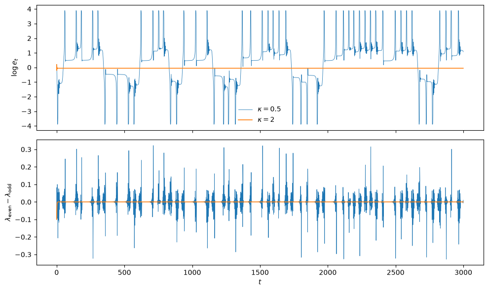
With the lecture’s tuning the learner does not converge.
The two classes’ portfolio shares nearly merge, saving reaches \(s^\star = 5\), and the exchange rate rests for a while.
Then the gap between the classes’ shares grows in an alternating pattern until it explodes.
The exchange rate shoots to the bounds and comes back to rest somewhere else, again and again.
For part 2, let \(\delta\) be the young class’s share minus the old class’s.
The portfolio return is \(A = \lambda_{\text{old}} R_1 + (1 - \lambda_{\text{old}}) R_2 = s_{\text{young}}/s_{\text{old}}\), which does not involve the shares.
So the saving equations do not involve \(\lambda\) at all.
Near a rest point, the cross term \(\partial^2 U/\partial s \partial \lambda\) is proportional to \(R_1 - R_2\) and vanishes.
The curvature estimate’s \(\lambda\) entry is then \(-\kappa\), and the old class’s update is
Next period the classes swap roles, so the new young-minus-old difference is \(-(1 - a)\delta\).
Measured as even minus odd, the gap is multiplied by \(1 - a\) at each update, and by \((1 - a)^2\) over two periods.
That is the eigenvalue we met in The ghost of indeterminacy.
The gap dies out if \(0 < a < 2\) and explodes if \(a > 2\).
def a_coef(p, lam, κ=0.5, gain=0.3):
    return gain * p.s_star / (κ * (p.w2 + p.s_star) * lam * (1 - lam))


for p, name in [(kw, "Sargent"), (arifovic, "Arifovic")]:
    for lam in (0.3, 0.5, 0.7):
        a = a_coef(p, lam)
        ev = np.sort(np.abs(np.linalg.eigvals(rest_point_jacobian(p, lam))))[::-1]
        print(f"{name:8s} λ = {lam}:  a = {a:.3f},  (1-a)² = {(1 - a)**2:.3f},  "
              f"|eigenvalues| = {ev.round(3)}")
Sargent  λ = 0.3:  a = 0.408,  (1-a)² = 0.350,  |eigenvalues| = [1.   0.35 0.25 0.16]
Sargent  λ = 0.5:  a = 0.343,  (1-a)² = 0.432,  |eigenvalues| = [1.    0.432 0.25  0.16 ]
Sargent  λ = 0.7:  a = 0.408,  (1-a)² = 0.350,  |eigenvalues| = [1.   0.35 0.25 0.16]
Arifovic λ = 0.3:  a = 2.381,  (1-a)² = 1.907,  |eigenvalues| = [1.907 1.    0.695 0.646]
Arifovic λ = 0.5:  a = 2.000,  (1-a)² = 1.000,  |eigenvalues| = [1.    1.    0.695 0.646]
Arifovic λ = 0.7:  a = 2.381,  (1-a)² = 1.907,  |eigenvalues| = [1.907 1.    0.695 0.646]
The formula matches the numerical Jacobian.
At Sargent’s parameters \(a\) is far below \(2\) unless \(\lambda\) is below about \(0.05\) or above about \(0.95\), so the rest points are stable apart from the unit eigenvalue along the continuum.
At Arifovic’s parameters the λ-gradient is much steeper, because the ratio \(s^\star/c_2^\star\) is \(5/6\) instead of \(1/7\).
With \(\kappa = 0.5\) and \(\gamma = 0.3\), then, \(a = 0.5/(\lambda(1-\lambda)) \geq 2\) at every rest point.
The rest point at \(\lambda = 1/2\) is exactly on the edge, and all the others are unstable.
That is why the learner keeps escaping.
For part 3, \(\lambda(1 - \lambda) \leq 1/4\), so some rest points are stable if and only if \(\kappa > 2\gamma s^\star / c_2^\star = 0.5\) at Arifovic’s parameters.
The lecture’s \(\kappa\) sits exactly on that boundary.
With \(\kappa = 2\) the rest points with \(\lambda(1-\lambda) > 1/16\), that is, with \(\lambda\) between about \(0.07\) and \(0.93\), are stable, and the figure shows the learner converging to a constant.
print(f"κ = 2: e → {eb[-1]:.4f},  s → {sb[-1].round(3)},  λ → {lb[-1].round(4)}")
print(f"largest |Δ log e| over the last 500 periods: "
      f"{np.abs(np.diff(np.log(eb[-500:]))).max():.1e}")
κ = 2: e → 0.9475,  s → [5. 5.],  λ → [0.5135 0.5135]
largest |Δ log e| over the last 500 periods: 0.0e+00
So the gap between the two halves of the lecture is about the adaptive machinery, not the calibration.
A Newton–Raphson learner that is damped enough converges at Arifovic’s parameters too, to a history-dependent constant.
But how much damping is “enough” depends on the economy: with the same tuning, one calibration converges and the other bursts.
Exercise 93.5
In a footnote, Sargent distinguishes history dependence from path dependence.
In a stochastic version of the model, realizations that start from identical initial conditions can converge to different exchange rates, because different shocks hit the transient dynamics.
Add IID shocks to the old-age endowment, \(w_{2t} = w_2 + \sigma \varepsilon_t\) with \(\varepsilon_t \sim N(0, 1)\) and \(\sigma = 1\), at Sargent’s parameters.
(The w2_path argument of newton_learning does this.)
Start \(200\) economies at the same initial condition, \(s_0 = (3.0, 2.2)\) and \(\lambda_0 = (0.30, 0.50)\), with different shock sequences, and run each for \(600\) periods. Does the exchange rate converge in each run? Does saving?
Plot a histogram of the limiting exchange rates, and mark the limit without shocks.
Why do the shocks stop affecting the exchange rate after a while, even though they never stop hitting the economy?
Solution
Here are parts 1 and 2.
T, σ = 600, 1.0
e_det = newton_learning(kw, [3.0, 2.2], [0.30, 0.50], T=T)[0][-1]

limits, last_move, s_spread = [], [], []
for seed in range(200):
    shocks = σ * np.random.default_rng(seed).standard_normal(T)
    e, s_h, l_h = newton_learning(kw, [3.0, 2.2], [0.30, 0.50], T=T,
                                  w2_path=kw.w2 + shocks)
    limits.append(e[-1])
    last_move.append(np.abs(np.diff(np.log(e[-300:]))).max())
    s_spread.append(s_h[-300:, 0].std())

fig, ax = plt.subplots(figsize=(7, 4))
ax.hist(limits, bins=30, alpha=0.7)
ax.axvline(e_det, color='k', ls='--', lw=1, label="no shocks")
ax.set_xlabel("limiting exchange rate")
ax.legend(frameon=False)
plt.show()
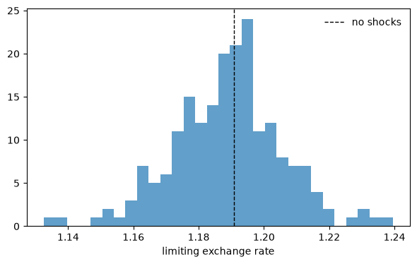
Here is a summary of the runs.
limits = np.array(limits)
print(f"limit without shocks: {e_det:.4f}")
print(f"limits with shocks: {limits.min():.4f} to {limits.max():.4f}, s.d. {limits.std():.4f}")
print(f"largest |Δ log e| over the last 300 periods, across all runs: {max(last_move):.1e}")
print(f"s.d. of even-class saving over the last 300 periods: "
      f"{min(s_spread):.3f} to {max(s_spread):.3f}")
limit without shocks: 1.1908
limits with shocks: 1.1326 to 1.2395, s.d. 0.0169
largest |Δ log e| over the last 300 periods, across all runs: 7.8e-16
s.d. of even-class saving over the last 300 periods: 0.193 to 0.274
Every exchange rate path converges: over the last \(300\) periods it does not move at all, up to rounding.
Saving does not converge; with a constant gain and shocks that never stop, it keeps fluctuating around \(s^\star\).
Yet the economies, which differ only in their shocks, settle on different exchange rates.
That is path dependence in Sargent’s sense.
Sargent [1993] quotes Evans and Honkapohja’s description of how adaptive learning resolves indeterminacy:
models with multiple solutions are converted into models with path dependence in which the trajectory of the economy, and the [rational expectations equilibrium] attained in the limit, are determined through a learning rule by initial forecasts and by the sequence of exogenous shocks.
The shocks matter only during the transient, because the exchange rate depends only on the young class’s \(\lambda\).
Once the two classes’ shares merge, \(R_1 = R_2\) whatever saving does, so the \(\lambda\)-gradient \(s(R_1 - R_2)/c_2\) is zero whatever the endowment.
From then on, shocks to \(w_2\) move saving but cannot move the portfolio share, and the exchange rate stays wherever the transient left it.
Because the shocks have only the brief transient in which to act, the spread of limits around the no-shock value is narrow.