95. Money as a Medium of Exchange among Artificially Intelligent Agents

95.1. Overview

Kiyotaki and Wright [Kiyotaki and Wright, 1989] studied an economy in which there is no double coincidence of wants.

Trade can occur only if some good is accepted not because it is wanted, but because it can be passed along later.

A good that plays that role is a medium of exchange.

Kiyotaki and Wright characterized stationary Nash equilibria of such an economy under the assumption that agents are fully rational: agents know the distribution of goods across their trading partners and best-respond to it.

Marimon, McGrattan and Sargent [Marimon et al., 1990] asked a different question.

Suppose we drop rationality altogether and put in its place a collection of artificially intelligent agents who begin with arbitrary, even random, rules of thumb, and who adapt those rules only by keeping score of what has paid off in the past.

Will such agents learn to use a medium of exchange?

And when the economy has two equilibria, or when its only equilibrium asks agents to be patient, what will they settle on?

These are instances of the question that A Peculiar Definition of Bounded Rationality asked of rational expectations (The knowledge that rational expectations imputes): can adaptive agents find an equilibrium, and which one?

The learning device that Marimon, McGrattan and Sargent used is John Holland’s classifier system [Holland, 1975, Holland et al., 1986].

Networks, Genetic Algorithms, and Classifier Systems introduced classifier systems and the bucket brigade in the abstract; here they are assembled into agents.

Each type of agent gets a population of if-then rules, an auction that decides which rule acts, and an accounting system that credits rules that lead to good outcomes and debits rules that lead to bad ones.

When the rules are generated at random, a genetic algorithm breeds new rules and retires old ones.

This lecture rebuilds their computational experiments and runs each of them for many random seeds, so that we can say how often each outcome occurs.

The main findings are:

1. With a complete list of rules, agents in Economy A1 learn its unique stationary equilibrium in every run: good 1, the cheapest good to store, circulates as money. Starting from random rules they get most of the way, as in the paper.

2. In Economy A2, where patient agents would speculate by accepting an expensive good, the artificial agents never do. Most runs settle on the fundamental pattern of trade, which is not an equilibrium of that economy, some only after thousands of periods stuck in a pattern with too little trade, and a few stay stuck for good. We show why: the bucket brigade makes the agents behave as if they discounted the future at a factor of about \(0.016\).

3. In Economy B, which has a fundamental and a speculative equilibrium, the agents select the fundamental one in most runs and the speculative one in none.

4. In nearly every run, an intrinsically worthless, costlessly stored object – fiat money – is accepted in trade by agents who have to discover its usefulness for themselves.

5. In an economy with five goods and five types, for which the authors had no analytical characterization of equilibrium, the algorithm proposes a pattern of trade, with qualifications that we describe.

Let’s start with some imports.

import numpy as np
import pandas as pd
import matplotlib.pyplot as plt
from dataclasses import dataclass, replace
from typing import NamedTuple
from numba import njit

95.2. The Kiyotaki-Wright environment

There are three types of agents, indexed by \(i = 1, 2, 3\), and three goods, indexed by \(k = 1, 2, 3\).

A type \(i\) agent derives utility only from consuming good \(i\).

He has a technology for producing good \(i^*\), where \(i^* \neq i\).

In Kiyotaki and Wright’s model A, the production pattern is the “Wicksell triangle”

type \(i\)	produces \(i^*\)	consumes
1	2	1
2	3	2
3	1	3

so there is no double coincidence of wants: the agent who has what you want never wants what you have.

All goods are indivisible and each agent can store exactly one unit of exactly one good from one period to the next.

Storing good \(k\) for one period costs \(s_k\), with

\[ s_3 > s_2 > s_1 > 0 . \]

There are equal numbers \(A_i\) of agents of each type, so \(A = 3 A_i\) in total.

Each period every agent is randomly matched with exactly one other agent, without regard to type.

Write \(x_{at}\) for the good that agent \(a\) carries into date \(t\) and \(\rho_t(a)\) for the agent with whom \(a\) is matched.

The pre-trade state of agent \(a\) is the pair

\[ z_{at} = \bigl(x_{at},\; x_{\rho_t(a)t}\bigr) . \]

Each period each agent makes two decisions in sequence.

First, having seen \(z_{at}\), he decides whether to propose a trade,

\[\begin{split} \lambda_{at} = \begin{cases} 1 & \text{propose to trade } x_{at} \text{ for } x_{\rho_t(a)t} \\ 0 & \text{refuse} \end{cases} \end{split}\]

Trade occurs if and only if \(\lambda_{at} \lambda_{\rho_t(a)t} = 1\), so post-trade holdings are

(95.1)\[x^+_{at} = (1 - \lambda_{at}\lambda_{\rho_t(a)t}) x_{at} + \lambda_{at}\lambda_{\rho_t(a)t} x_{\rho_t(a)t} .\]

Second, he decides whether to consume what he is left holding,

\[\begin{split} \gamma_{at} = \begin{cases} 1 & \text{consume } x^+_{at} \\ 0 & \text{carry } x^+_{at} \text{ into } t+1 \end{cases} \end{split}\]

If he consumes he immediately produces good \(f(a) = i^*\) and carries that into \(t+1\).

Hence

(95.2)\[x_{a,t+1} = \gamma_{at} f(a) + (1 - \gamma_{at}) x^+_{at} .\]

The one-period net payoff is

(95.3)\[U_a(\gamma_{at}) = \gamma_{at}\bigl[u_i(x^+_{at}) - s(f(a))\bigr] - (1 - \gamma_{at})\, s(x^+_{at}) ,\]

where \(u_i(k) = u_i > 0\) if \(k = i\) and \(u_i(k) = 0\) otherwise.

Note that an agent is permitted to consume a good he does not want; he simply gets zero utility from it while still producing and paying to store \(f(a)\).

This “consume anything” feature has a consequence worth stating once.

An agent who swaps his own production good for some other good and then eats it ends the period exactly where refusing to trade would have left him: holding his production good and paying its storage cost.

Such trades are payoff-neutral, so nothing in the accounting system described below pushes them out, and they will turn up in several of our economies.

Note

Kiyotaki and Wright ranked payoff streams by expected discounted utility.

Marimon, McGrattan and Sargent instead assume that each agent cares about his long-run average utility, and they build the accounting system inside a classifier system out of running averages for that reason.

We shall see in The bucket brigade’s discount factor that the agents this accounting system produces nevertheless behave as if they discounted the future very heavily.

95.2.1. Two equilibria

Since agents’ payoffs depend on what other agents do, the model can have more than one stationary equilibrium.

Kiyotaki and Wright characterize equilibria by a set of probabilities, of which the most useful for us is

\[ \pi^h_{it}(k) = \text{probability that a type } i \text{ agent holds good } k \text{ at } t . \]

In the fundamental equilibrium, good 1 – the cheapest to store – is the general medium of exchange:

• type 1 agents always hold good 2 (which they produce) and trade it for good 1;

• type 3 agents always hold good 1 and trade it for good 3;

• type 2 agents hold good 1 half the time and good 3 half the time.

So the equilibrium holding probabilities are

	\(k=1\)	\(k=2\)	\(k=3\)
\(i=1\)	0	1	0
\(i=2\)	0.5	0	0.5
\(i=3\)	1	0	0

Type 2 agents accept good 1 even though they never consume it: they use it as money.

In the speculative equilibrium, type 1 agents additionally accept good 3 – the most expensive good to store – because they expect to trade it away quickly for good 1.

The reason is that a type 1 agent holding good 2 can get good 1 only from a type 2 agent, whereas a type 1 agent holding good 3 can get it from a type 3 agent, who wants good 3 and holds good 1.

Each partner type is met with probability \(1/3\), so holding good 3 instead of good 2 raises the chance of acquiring good 1 each period by \(\bigl(\pi^h_3(1) - \pi^h_2(1)\bigr)/3\), at an extra storage cost of \(s_3 - s_2\).

Kiyotaki and Wright show that, in the limit as the discount rate goes to zero, the fundamental equilibrium is the unique stationary equilibrium if

(95.4)\[s_3 - s_2 > \bigl(\pi^h_3(1) - \pi^h_2(1)\bigr)\tfrac{1}{3} u_1 ,\]

evaluated at fundamental holdings, and that the speculative equilibrium is the unique one when the inequality is reversed at speculative holdings.

Footnote 7 of the paper prints \(\pi^h_1(3) - \pi^h_1(2)\), which transposes the indices: with type 1’s own holdings the right side would be \(-u_1/3\) and the inequality could never fail.

At the fundamental equilibrium \(\pi^h_3(1) = 1\) and \(\pi^h_2(1) = 1/2\), and at the speculative equilibrium (tabulated below) \(\pi^h_2(1) = 0.586\).

The following function solves (95.4) for \(u_1\); the argument \(\beta\) will be used in The bucket brigade’s discount factor.

s_A = np.array([0.1, 1.0, 20.0])           # storage costs in Economy A


def speculation_threshold(s, π31, π21, β=1.0):
    "The u_1 above which a type 1 agent with discount factor β prefers good 3."
    return 3 * (s[2] - s[1]) / (β * (π31 - π21))


u_fund = speculation_threshold(s_A, π31=1.0, π21=0.5)     # at fundamental holdings
u_spec = speculation_threshold(s_A, π31=1.0, π21=0.586)   # at speculative holdings
print(f"fundamental equilibrium requires u_1 < {u_fund:.1f}")
print(f"speculative equilibrium requires u_1 > {u_spec:.1f}")

fundamental equilibrium requires u_1 < 114.0
speculative equilibrium requires u_1 > 137.7

Economy A1 has \(u_1 = 100\), which satisfies the fundamental condition, though the cutoff is only 14 percent above it.

Economy A2 has \(u_1 = 500\), which violates it, so for patient agents the unique stationary equilibrium of A2 is the speculative one.

Each of these economies thus has one stationary equilibrium for patient agents, and the question it poses is whether that equilibrium is learnable.

Economy B below has two, and poses the question of selection.

95.2.2. The economies

The following table, modeled on the paper’s Table 4, lists the economies we simulate.

All have fifty agents of each type and equal utilities \(u_i = u\) for every type.

economy	type \(i\) produces	storage costs	\(u\)	bids \(b_{11}, b_{12}, b_{21}, b_{22}\)	initial rules	equilibrium for patient agents
A1.1	2, 3, 1	0.1, 1, 20	100	0.025, 0.025, 0.25, 0.25	all 72 + 12	fundamental
A2.1	2, 3, 1	0.1, 1, 20	500	0.025, 0.025, 0.25, 0.25	all 72 + 12	speculative
B.1	3, 1, 2	1, 4, 9	100	0.25, 0.25, 0.25, 0.25	all 72 + 12	fundamental and speculative
A1.2	2, 3, 1	0.1, 1, 20	100	0.025, 0.025, 0.25, 0.25	72 + 12 random	fundamental
A2.2	2, 3, 1	0.1, 1, 20	500	0.025, 0.025, 0.25, 0.25	72 + 12 random	speculative
B.2	3, 1, 2	1, 4, 9	100	0.025, 0.025, 0.25, 0.25	72 + 12 random	fundamental and speculative
C	2, 3, 1	9, 14, 29; fiat 0	100	0.025, 0.025, 0.025, 0.25	150 + 20 random	fundamental
D	3, 4, 5, 1, 2	1, 4, 9, 20, 30	200	0.025, 0.025, 0.25, 0.25	180 + 20 random	not characterized

The bids are explained below; “all 72 + 12” means a complete enumeration of exchange and consumption rules.

A2.2 and B.2 appear in the exercises.

The paper’s Table 4 lists Economy C’s storage costs as 0.1, 20 and 70, but its Table 15, which reports the simulation, lists 9, 14 and 29, and we use those.

95.3. Classifier systems for the Kiyotaki-Wright environment

Networks, Genetic Algorithms, and Classifier Systems set out the general machinery in Classifier systems: the alphabet \(\{0, 1, \#\}\), matching, specificity, and auctions among rules with strengths.

Its The bucket brigade showed how a rule that sets up a later reward gets paid for it.

Here we record only what is specific to Marimon, McGrattan and Sargent: how goods are encoded, the two decisions each agent makes every period, and the two strength equations that link them.

95.3.1. Encoding

Each type has two classifier systems, one for exchange decisions and one for consumption decisions.

The paper’s Table 1 encodes goods with three positions each: a one-hot code for “good \(k\)” and a code with a \(0\) in position \(k\) for “not good \(k\)”.

WILD = -1                                   # the "don't care" symbol #


def table1(n_goods):
    "The paper's Table 1: one-hot codes for 'good k', then codes for 'not good k'."
    good = np.eye(n_goods, dtype=np.int8)
    not_good = np.full((n_goods, n_goods), WILD, dtype=np.int8)
    np.fill_diagonal(not_good, 0)
    return np.vstack([good, not_good])


def code_string(c):
    return ''.join('#' if b == WILD else str(int(b)) for b in c)


def rule_string(cond, action, n_goods):
    "Print a classifier the way the paper does, for example '010 100 -> 1'."
    s = code_string(cond)
    if len(cond) == 2 * n_goods:
        s = s[:n_goods] + ' ' + s[n_goods:]
    return f"{s} -> {int(action)}"


pd.DataFrame({'code': [code_string(c) for c in table1(3)],
              'meaning': [f'good {k}' for k in (1, 2, 3)]
                         + [f'not good {k}' for k in (1, 2, 3)]})

	code	meaning
0	100	good 1
1	010	good 2
2	001	good 3
3	0##	not good 1
4	#0#	not good 2
5	##0	not good 3

An exchange classifier is a string of length 7: three positions for the agent’s own holding, three for the partner’s holding, and a binary action (\(1\) = propose trade, \(0\) = refuse).

The paper’s two examples are

100 001 -> 1     "if I hold good 1 and my partner holds good 3, propose to trade"
100 ##0 -> 0     "if I hold good 1 and my partner does not hold good 3, refuse"

A consumption classifier is a string of length 4: three positions for the post-trade holding \(x^+_{at}\) and one action digit (\(1\) = consume).

A complete enumeration pairs every condition in Table 1 with both actions.

That gives \(6 \times 6 \times 2 = 72\) exchange classifiers and \(6 \times 2 = 12\) consumption classifiers, enough to express every Markov strategy.

Table 1 has no condition meaning “any good”, so the enumeration contains no rule such as “eat whatever you hold”.

When rules are drawn at random, each position is \(0\), \(1\) or \(\#\) with equal probability.

There are then \(3^6 \times 2 = 1458\) possible exchange strings and \(3^3 \times 2 = 54\) consumption strings, and many of them match no state at all: 110, for instance, is no good’s code.

With four objects (Economy C) or five goods (Economy D) the codes are one-hot strings of length four or five.

For C that gives the paper’s count of \(3^8 \times 2 = 13{,}122\) possible exchange strings.

The paper does not say how it encoded the goods of Economy D, so the five-position code is our choice.

A rule’s specificity is \(\sigma = 1/(1 + \text{number of } \#\text{'s})\).

An exchange rule about two particular goods has \(\sigma = 1\), a rule like 100 ##0 has \(\sigma = 1/3\), and a rule about two “not” conditions has \(\sigma = 1/5\).

95.3.2. The auction

Attached to classifier \(e\) at date \(t\) is a strength \(S^a_e(t)\).

Given the state \(z_{at}\), let \(M_e(z_{at})\) be the set of exchange classifiers whose conditions \(z_{at}\) satisfies.

The classifier that acts is the strongest matched one,

(95.5)\[e_t(z_{at}) = \arg\max\,\{S^a_e(t) : e \in M_e(z_{at})\} ,\]

and the consumption classifier is chosen the same way from the classifiers that match \(x^+_{at}\).

This is the paper’s equation (6); we break ties at random, a detail the paper does not specify.

Each matched classifier also has a bid, a fraction of its strength,

\[ b_1(e) = b_{11} + b_{12}\sigma_e \qquad\text{and}\qquad b_2(c) = b_{21} + b_{22}\sigma_c \]

for exchange and consumption classifiers, respectively.

Under (95.5) the bid plays no role in deciding who wins: it only determines the payments described below.

The paper’s verbal description calls the winner “the highest bidder” and says that bids that rise with specificity “favor specific rules over more general rules”.

That would be true of an auction on \(b \cdot S\) among rules of positive strength, but under (95.5) a larger bid fraction pulls a rule’s strength at a rest point toward zero, as the note below shows.

So among rules whose downstream payments are positive, higher bids lower stationary strength and favor general rules; only among rules whose downstream payments are negative do they favor specific rules, as the paper says.

The argmax auction is the greedy limit of the softmax auction in Networks, Genetic Algorithms, and Classifier Systems’s two-armed bandit exercise (Exercise 94.3), in which matched rule \(r\) wins with probability proportional to \(e^{\eta S_r}\) and \(\eta \to \infty\) gives the argmax; that lecture calls the intensity \(\beta\), a letter we reserve here for discount factors.

The paper’s footnote 5 mentions such a stochastic auction as an alternative.

A greedy auction avoids probability matching, but it leaves all experimentation to the initial strengths and to the operators that create new rules, a choice that will matter in Economy A2.

95.3.3. The bucket brigade

Strengths are updated by a system of internal payments that Holland calls a bucket brigade.

Only the classifier that wins an auction changes its strength, so each classifier carries a counter \(\tau^a_e(t)\) recording the number of auctions it has won, initialized at 1.

Payments flow as follows.

• The external payoff \(U_a(\gamma_t)\) goes to the winning consumption classifier at \(t\).

• The winning consumption classifier at \(t\) pays its bid to the winning exchange classifier at \(t\), which created the state that gave it a chance to act.

• The winning exchange classifier at \(t\) pays its bid to the winning consumption classifier at \(t-1\), which set up the state \(z_{at}\).

The resulting laws of motion are the paper’s equations (12) and (13),

(95.6)\[S^a_{c,\tau_c(t)} = S^a_{c,\tau_c(t)-1} - \frac{1}{\tau_c(t)-1}\Bigl[(1 + b_2(c))S^a_{c,\tau_c(t)-1} - \sum_e I^a_e(t) b_1(e) S^a_{e,\tau_e(t)} - U_a(\gamma_{ct})\Bigr]\]

(95.7)\[S^a_{e,\tau_e(t)+1} = S^a_{e,\tau_e(t)} - \frac{1}{\tau_e(t)}\Bigl[(1 + b_1(e))S^a_{e,\tau_e(t)} - \sum_c I^a_c(t) b_2(c) S^a_{c,\tau_c(t)}\Bigr]\]

where \(I^a_e(t)\) and \(I^a_c(t)\) are indicators for winning the auction at \(t\).

So the consumption classifier updated at date \(t\) is the one that won at \(t-1\), and each bid travels one step back along the chain

\[ \cdots \;\to\; c_{t-1} \;\to\; e_t \;\to\; c_t \;\to\; e_{t+1} \;\to\; \cdots \]

An exchange classifier that proposes a trade which is not reciprocated is not charged, its counter does not advance, and it pays nothing backward: the agent learns nothing from an offer that was refused.

All agents of a given type share one classifier system, as in the paper.

The paper runs (95.6)-(95.7) in “synthetic time”, counting matches rather than periods, so read literally a consumption classifier is paid by the next exchange classifier of its type to act, which usually belongs to a different agent.

We instead link each agent’s own consecutive decisions, which is what the equations describe for a single agent, and the reading under which a decision is credited with its own consequences.

Note

Equations (95.6)-(95.7) make strength a running average of past net receipts rather than a cumulative total, which is what Holland’s original specification used; the paper’s footnote 8 says the averaging was chosen so that strengths could converge.

With \(1/\tau\) gains these are stochastic approximation recursions, the same decreasing-gain recursion that drives the learners of Adaptive Agents in an Overlapping Generations Monetary Economy and Learning, Approximation, and Equilibrium Computation (One recursion, many learners).

So any limit point must satisfy the paper’s equation (17),

\[ \mathbb{E}\Bigl[(1 + b_2(c))S_c - \sum_e I_e b_1(e) S_e - U(\gamma_c)\Bigr] = 0, \qquad \mathbb{E}\Bigl[(1 + b_1(e))S_e - \sum_c I_c b_2(c) S_c\Bigr] = 0 . \]

Marimon, McGrattan and Sargent call strengths solving these equations stationary, and say a stationary Nash equilibrium is supported when the rules that win auctions at stationary strengths are exactly the rules that implement equilibrium behavior.

The second equation gives \(S_e = \mathbb{E}[b_2(c) S_c]/(1 + b_1(e))\), so a larger bid fraction \(b_1(e)\) shrinks a rule’s stationary strength toward zero: it lowers \(S_e\) when \(\mathbb{E}[b_2(c) S_c] > 0\) and raises it when \(\mathbb{E}[b_2(c) S_c] < 0\).

One more feature of the system drives much of what follows.

All strengths start at zero, while nearly every net payoff an agent experiences is negative, because storage is costly.

So an untried rule beats every rule whose experience so far has been net costly, and under the argmax auction an agent sweeps through its untried rules early on.

This optimistic initialization is the main way an agent experiments when it starts from a complete enumeration.

It has a failure mode.

A rule that has never acted, or whose offers were all refused so that it learned nothing, keeps its strength of zero, and it loses every auction to a rival whose strength happens to sit slightly above zero, for as long as that rival’s average stays there.

95.4. Implementation

The state spaces are tiny, so for every rule we precompute the set of states it matches and store it as the bits of an integer: state \((x, y)\) of an exchange rule is bit \(x G + y\), where \(G\) is the number of goods.

The simulation loops run under Numba’s njit.

Classifier systems are stored as parallel arrays indexed by type and rule.

class Rules(NamedTuple):
    "Classifier systems for all types, stored as arrays indexed [type, rule]."
    cond: np.ndarray        # condition part, entries in {0, 1, WILD}
    action: np.ndarray      # action part: 1 = trade (or consume), 0 = refuse
    strength: np.ndarray    # S, a running average of net receipts
    used: np.ndarray        # the counter tau, initialized at 1
    match: np.ndarray       # bit s is set if the rule matches state s
    sigma: np.ndarray       # specificity, 1 / (1 + number of #'s)
    born: np.ndarray        # a stamp that changes whenever the rule is replaced


@njit
def goods_matched(field):
    "Bitmask of the goods whose one-hot code satisfies a condition field."
    n_goods = field.shape[0]
    mask = 0
    for g in range(n_goods):
        ok = True
        for j in range(n_goods):
            if field[j] != WILD and field[j] != (1 if j == g else 0):
                ok = False
        if ok:
            mask |= 1 << g
    return mask


@njit
def refresh(R, i, r, n_goods):
    "Record which states rule r of type i matches, and its specificity."
    c = R.cond[i, r]
    if c.shape[0] == n_goods:                    # consumption rule: state = holding
        m = goods_matched(c)
    else:                                        # exchange rule: state = (own, partner)
        own, partner = goods_matched(c[:n_goods]), goods_matched(c[n_goods:])
        m = 0
        for x in range(n_goods):
            for y in range(n_goods):
                if (own >> x) & 1 and (partner >> y) & 1:
                    m |= 1 << (x * n_goods + y)
    R.match[i, r] = m
    R.sigma[i, r] = 1.0 / (1.0 + np.sum(c == WILD))


@njit
def set_rule(R, i, r, cond, action, strength, n_goods, stamp):
    "Overwrite rule r of type i with a new classifier, whose counter starts at 1."
    R.cond[i, r] = cond
    R.action[i, r] = action
    R.strength[i, r] = strength
    R.used[i, r] = 1
    stamp[0] += 1
    R.born[i, r] = stamp[0]
    refresh(R, i, r, n_goods)

A complete enumeration pairs every condition in Table 1 with both actions, while a random population draws every position independently.

Following the paper, all initial strengths are zero.

def make_rules(cond, action, n_goods):
    n_types, n = action.shape
    R = Rules(cond.astype(np.int8), action.astype(np.int8),
              np.zeros((n_types, n)), np.ones((n_types, n), np.int64),
              np.zeros((n_types, n), np.int64), np.zeros((n_types, n)),
              np.zeros((n_types, n), np.int64))
    for i in range(n_types):
        for r in range(n):
            refresh(R, i, r, n_goods)
    return R


def complete_rules(n_types, n_goods, exchange, specific_only=False):
    "Every Table 1 condition (or pair of conditions) with both actions."
    conds = table1(n_goods)[:n_goods] if specific_only else table1(n_goods)
    if exchange:
        conds = np.array([np.concatenate([a, b]) for a in conds for b in conds])
    cond = np.tile(np.repeat(conds, 2, axis=0), (n_types, 1, 1))
    action = np.tile([0, 1], (n_types, len(conds)))
    return make_rules(cond, action, n_goods)


def random_rules(n_types, n_rules, length, n_goods, rng):
    "Rules whose positions are drawn independently and uniformly from {0, 1, #}."
    return make_rules(rng.integers(-1, 2, size=(n_types, n_rules, length)),
                      rng.integers(0, 2, size=(n_types, n_rules)), n_goods)

The auction (95.5) follows.

For the exercises it also offers the softmax auction with intensity \(\eta\).

Several operators below must delete a “weak” rule, and the paper measures weakness “in terms of a combination of strength and cumulated number of times the classifier has won the bidding in the past”.

Our combination adds the two, each rescaled to \([0, 1]\) across the candidates.

@njit
def auction(R, i, s, eta, rng):
    """
    The rule of type i that decides in state s, or -1 if no rule matches.

    eta = inf is the paper's auction: the strongest matched rule wins, with
    ties broken at random.  A finite eta gives a softmax auction instead.
    """
    S, match = R.strength[i], R.match[i]
    best, top, n_ties = -1, -np.inf, 0
    for r in range(S.shape[0]):
        if (match[r] >> s) & 1:
            if S[r] > top:
                best, top, n_ties = r, S[r], 1
            elif S[r] == top:
                n_ties += 1
                if rng.random() * n_ties < 1:
                    best = r
    if best < 0 or eta == np.inf:
        return best
    total = 0.0
    for r in range(S.shape[0]):
        if (match[r] >> s) & 1:
            total += np.exp(eta * (S[r] - top))
    x = rng.random() * total
    for r in range(S.shape[0]):
        if (match[r] >> s) & 1:
            x -= np.exp(eta * (S[r] - top))
            if x <= 0:
                return r
    return best


@njit
def weakest(R, i, s, exclude):
    """
    The weakest rule of type i other than `exclude`, scoring each candidate by
    its strength plus its number of wins, each rescaled to [0, 1].  Candidates
    are the rules matching state s, or all rules if none does or if s < 0.
    """
    S, used, match = R.strength[i], R.used[i], R.match[i]
    n = S.shape[0]
    cand = np.zeros(n, np.bool_)
    for r in range(n):
        cand[r] = r != exclude and (s < 0 or ((match[r] >> s) & 1) == 1)
    if not cand.any():
        for r in range(n):
            cand[r] = r != exclude
    lo, hi = S[cand].min(), S[cand].max()
    u_lo, u_hi = used[cand].min(), used[cand].max()
    best, best_score = -1, np.inf
    for r in range(n):
        if cand[r]:
            score = ((S[r] - lo) / (hi - lo + 1e-12)
                     + (used[r] - u_lo) / (u_hi - u_lo + 1e-12))
            if score < best_score:
                best, best_score = r, score
    return best

Three of the four operators that the paper adds for random rules (its Section 6) act inside an auction, so we implement them here.

Creation fires when no rule matches the state: the weakest rule is replaced by one whose condition is exactly the state, with a random action.

Diversification fires when every matched rule calls for the same action: the weakest other matched rule is replaced by a rule for exactly this state with the opposite action and the winner’s strength, which then ties with the winner.

Specialization is switched on in period \(t\) with probability \(f_s(t) = 1/(2\sqrt{t})\).

When it is on, each \(\#\) in the winner’s condition is replaced, with probability \(p_s = 0.01\), by the bit that matches the current state, and the sharpened copy replaces a weak matched rule.

Under a complete enumeration every state is matched and every condition appears with both actions, so creation and diversification never fire, as the paper notes; specialization is used only with random rules.

@njit
def decide(R, i, s, code, eta, specialize, ps, n_goods, rng, stamp):
    """
    Run the auction of type i in state s, whose encoding is `code`, applying
    the paper's creation, diversification and specialization operators.
    """
    w = auction(R, i, s, eta, rng)
    if w < 0:                                          # creation
        j = weakest(R, i, -1, -1)
        set_rule(R, i, j, code, rng.integers(0, 2), 0.0, n_goods, stamp)
        return j

    one_action = True                                  # diversification
    for r in range(R.action.shape[1]):
        if (R.match[i, r] >> s) & 1 and R.action[i, r] != R.action[i, w]:
            one_action = False
            break
    if one_action:
        j = weakest(R, i, s, w)
        set_rule(R, i, j, code, 1 - R.action[i, w], R.strength[i, w],
                 n_goods, stamp)
        w = auction(R, i, s, eta, rng)

    if specialize:                                     # specialization
        new = R.cond[i, w].copy()
        changed = False
        for k in range(new.shape[0]):
            if new[k] == WILD and rng.random() < ps:
                new[k] = code[k]
                changed = True
        if changed:
            j = weakest(R, i, s, w)
            set_rule(R, i, j, new, R.action[i, w], R.strength[i, w],
                     n_goods, stamp)
    return w

An Economy collects the parameters of the physical environment together with the settings of the learning algorithm.

Goods are numbered from 0 in the code and from 1 in the text, and fiat money, when present, is the last good.

The last three fields are used only in the exercises.

@dataclass
class Economy:
    name: str
    produces: np.ndarray               # produces[i] = good produced by type i
    storage_costs: np.ndarray          # one per good; fiat money, if any, is last
    u: float = 100.0                   # utility from consuming one's own good
    n_agents_per_type: int = 50
    random_rules: bool = False         # False: complete enumeration, no GA
    n_trade_rules: int = 72            # population sizes when rules are random
    n_consume_rules: int = 12
    b_trade: tuple = (0.025, 0.025)    # (b11, b12)
    b_consume: tuple = (0.25, 0.25)    # (b21, b22)
    n_fiat: int = 0                    # units of fiat money handed out at t = 0
    ps: float = 0.01                   # specialization: chance a # is filled in
    eta: float = np.inf                # inf: argmax auction; finite: softmax
    no_eat: bool = False               # True: only one's own good can be eaten
    specific_only: bool = False        # True: enumerate fully specific rules only

    @property
    def n_types(self):
        return len(self.produces)

    @property
    def n_goods(self):
        return len(self.storage_costs)

    @property
    def fiat(self):
        "Index of fiat money, or -1 if there is none."
        return self.n_goods - 1 if self.n_goods > self.n_types else -1

The bucket brigade updates two strengths for each agent each period: the exchange rule that won today, as in (95.7), and the consumption rule that won for the same agent yesterday, as in (95.6), whose second receipt is only now known.

The born stamps guard against paying a rule that has been overwritten in the meantime.

@njit
def bucket_brigade(E, C, i, a, e, active, c, payoff, b, pending):
    """
    Update strengths for agent a of type i: first the exchange rule e that
    won today, then the consumption rule that won for this agent yesterday.
    """
    b11, b12, b21, b22 = b
    last_c, last_payoff, last_born = pending
    S_e = E.strength[i, e]                        # before its own update
    b1 = b11 + b12 * E.sigma[i, e]
    if active:                                    # equation (13)
        tau = E.used[i, e]
        E.used[i, e] = tau + 1
        b2 = b21 + b22 * C.sigma[i, c]
        E.strength[i, e] = S_e - ((1 + b1) * S_e - b2 * C.strength[i, c]) / tau
    p = last_c[a]
    if p >= 0 and C.born[i, p] == last_born[a]:   # equation (12)
        inflow = b1 * S_e if active else 0.0
        b2p = b21 + b22 * C.sigma[i, p]
        tau = C.used[i, p]
        C.used[i, p] = tau + 1
        C.strength[i, p] -= ((1 + b2p) * C.strength[i, p]
                             - inflow - last_payoff[a]) / tau
    last_c[a], last_payoff[a], last_born[a] = c, payoff, C.born[i, c]

Each period all \(A\) agents are shuffled into \(A/2\) pairs, and each pair makes its exchange decisions, trades if both propose, makes its consumption decisions, and settles accounts.

@njit
def run_period(E, C, hold, types, produces, s, u, fiat, b, pending, eta,
               specialize, ps, no_eat, rng, stamp, exch, cons):
    "One period: random matching, two auctions per agent, and the accounting."
    n_goods = s.shape[0]
    order = rng.permutation(hold.shape[0])
    code = np.zeros(2 * n_goods, np.int8)
    e = np.zeros(2, np.int64)
    e_born = np.zeros(2, np.int64)
    offer = np.zeros(2, np.int64)
    for k in range(hold.shape[0] // 2):
        pair = (order[2 * k], order[2 * k + 1])
        x = (hold[pair[0]], hold[pair[1]])

        for m in range(2):                        # exchange decisions
            i = types[pair[m]]
            code[:] = 0
            code[x[m]] = 1
            code[n_goods + x[1 - m]] = 1
            e[m] = decide(E, i, x[m] * n_goods + x[1 - m], code, eta,
                          specialize, ps, n_goods, rng, stamp)
            e_born[m], offer[m] = E.born[i, e[m]], E.action[i, e[m]]
        trade = offer[0] == 1 and offer[1] == 1
        if trade:
            hold[pair[0]], hold[pair[1]] = x[1], x[0]
            exch[types[pair[0]], x[0], x[1]] += 1
            exch[types[pair[1]], x[1], x[0]] += 1

        for m in range(2):                        # consumption decisions
            a = pair[m]
            i, g = types[a], hold[a]
            code[:] = 0
            code[g] = 1
            c = decide(C, i, g, code[:n_goods], eta, specialize, ps,
                       n_goods, rng, stamp)
            cons[i, g, 0] += 1
            if C.action[i, c] == 1 and g != fiat and (not no_eat or g == i):
                cons[i, g, 1] += 1
                hold[a] = produces[i]
                payoff = (u if g == i else 0.0) - s[produces[i]]
            else:
                payoff = -s[g]
            active = (trade or offer[m] == 0) and E.born[i, e[m]] == e_born[m]
            bucket_brigade(E, C, i, a, e[m], active, c, payoff, b, pending)

A Simulation holds the state of an economy and runs it period by period, recording holdings, trades and consumption decisions.

Initial holdings are random, as in the paper, and fiat money is handed to randomly chosen agents.

With random rules, the genetic algorithm generalize runs after each period; it is defined in The genetic algorithm, before the first economy that needs it.

class Simulation:

    def __init__(self, econ, seed=0):
        self.econ = econ
        self.rng = rng = np.random.default_rng(seed)
        K, G = econ.n_types, econ.n_goods
        if econ.random_rules:
            self.E = random_rules(K, econ.n_trade_rules, 2 * G, G, rng)
            self.C = random_rules(K, econ.n_consume_rules, G, G, rng)
        else:
            self.E = complete_rules(K, G, True, econ.specific_only)
            self.C = complete_rules(K, G, False, econ.specific_only)
        self.types = np.repeat(np.arange(K), econ.n_agents_per_type)
        A = len(self.types)
        self.hold = rng.integers(0, K, size=A)       # random commodity holdings
        if econ.n_fiat:
            self.hold[rng.choice(A, econ.n_fiat, replace=False)] = econ.fiat
        self.pending = (np.full(A, -1), np.zeros(A), np.zeros(A, np.int64))
        self.stamp = np.zeros(1, np.int64)
        self.t = 0
        self.hold_hist, self.exch_hist, self.cons_hist = [], [], []

    def run(self, T):
        econ, rng = self.econ, self.rng
        K, G = econ.n_types, econ.n_goods
        b = tuple(float(v) for v in econ.b_trade + econ.b_consume)
        for _ in range(T):
            self.t += 1
            f = 1 / (2 * np.sqrt(self.t))   # rate of specialization and the GA
            specialize = econ.random_rules and rng.random() < f
            exch, cons = np.zeros((K, G, G)), np.zeros((K, G, 2))
            run_period(self.E, self.C, self.hold, self.types, econ.produces,
                       econ.storage_costs, econ.u, econ.fiat, b, self.pending,
                       econ.eta, specialize, econ.ps, econ.no_eat, rng,
                       self.stamp, exch, cons)
            if econ.random_rules:
                for i in range(K):
                    if rng.random() < f:
                        generalize(self.E, i, G, rng, self.stamp, n_crowd=8)
                    if rng.random() < f:
                        generalize(self.C, i, G, rng, self.stamp, n_crowd=4)
            self.hold_hist.append([np.bincount(self.hold[self.types == i],
                                               minlength=G) for i in range(K)])
            self.exch_hist.append(exch)
            self.cons_hist.append(cons)

The next cell defines helpers that put the output into the format of the paper’s tables (which report ten-period moving averages) and figures.

winners lists, for each state, the rule that would win the auction there, and contenders lists every rule competing in a state.

across_seeds reruns an economy for twenty seeds.

Show code cell source

Hide code cell source

def good_names(econ):
    names = [f"good {k+1}" for k in range(econ.n_types)]
    return names + ["fiat"] if econ.fiat >= 0 else names


def type_names(econ):
    return [f"type {i+1}" for i in range(econ.n_types)]


def holdings(sim, t=None, window=10):
    "Table of pi^h_i(k), averaged over the `window` periods ending at t."
    h = np.array(sim.hold_hist) / sim.econ.n_agents_per_type
    t = len(h) if t is None else t
    return pd.DataFrame(h[max(0, t - window):t].mean(axis=0),
                        index=type_names(sim.econ),
                        columns=good_names(sim.econ)).round(3)


def strongest(R, i, s):
    "Strongest rule of type i matching state s (ties go to the first), or -1."
    idx = np.flatnonzero((R.match[i] >> s) & 1)
    return -1 if idx.size == 0 else idx[np.argmax(R.strength[i, idx])]


def winners(sim, i, exchange=True):
    "The rule of type i that wins in each state, with its strength and uses."
    econ, G = sim.econ, sim.econ.n_goods
    R = sim.E if exchange else sim.C
    names = good_names(econ)
    states = ([(j, k) for j in range(G) for k in range(G)] if exchange
              else [(j,) for j in range(G)])
    rows = []
    for st in states:
        w = strongest(R, i, st[0] * G + st[1] if exchange else st[0])
        rows.append({'state': ', '.join(names[g] for g in st),
                     'winning rule': rule_string(R.cond[i, w], R.action[i, w], G),
                     'strength': round(R.strength[i, w], 2),
                     'times used': R.used[i, w] - 1})
    return pd.DataFrame(rows).set_index('state')


def eating_rates(sim, window=200):
    "Fraction of the time each type eats each good it holds after trading."
    c = np.array(sim.cons_hist[-window:]).sum(axis=0)
    rate = c[:, :, 1] / np.maximum(c[:, :, 0], 1)
    return pd.DataFrame(rate, index=type_names(sim.econ),
                        columns=good_names(sim.econ)).round(2)


def contenders(sim, i, j, k):
    "All exchange rules of type i matching the state (good j+1, good k+1), strongest first."
    G, R = sim.econ.n_goods, sim.E
    idx = np.flatnonzero((R.match[i] >> (j * G + k)) & 1)
    idx = idx[np.argsort(-R.strength[i, idx], kind='stable')]
    return pd.DataFrame({'rule': [rule_string(R.cond[i, r], R.action[i, r], G)
                                  for r in idx],
                         'strength': R.strength[i, idx].round(2),
                         'times used': R.used[i, idx] - 1})


def trade_rates(sim, window=100):
    "Trades per agent per period over the last `window` periods, indexed [type, gives, gets]."
    return np.array(sim.exch_hist[-window:]).mean(axis=0) / sim.econ.n_agents_per_type


def across_seeds(econ, T, seeds=range(20)):
    "Run the economy for T periods once for each seed."
    sims = []
    for seed in seeds:
        sim = Simulation(econ, seed)
        sim.run(T)
        sims.append(sim)
    return sims


def final_holdings(sims, t=None):
    "Holdings at t (ten-period averages) for each simulation, as an array."
    return np.array([holdings(sim, t=t).to_numpy() for sim in sims])


def distance(H, target):
    "Largest absolute difference between each run's holdings and a target table."
    return np.abs(H - np.asarray(target)).max(axis=(-2, -1))


def plot_holdings(sim):
    econ = sim.econ
    h = np.array(sim.hold_hist) / econ.n_agents_per_type
    names = good_names(econ)
    fig, axes = plt.subplots(1, econ.n_types, figsize=(3.2 * econ.n_types, 3.2),
                             sharey=True)
    for i, ax in enumerate(axes):
        for k in range(econ.n_goods):
            ax.plot(h[:, i, k], lw=1.0, label=names[k])
        ax.set_title(f"type {i+1}")
        ax.set_xlabel("$t$")
        ax.set_ylim(-0.03, 1.03)
    axes[0].set_ylabel(r"$\pi^h_{it}(k)$")
    fig.legend(*axes[0].get_legend_handles_labels(), loc='center right',
               frameon=False, fontsize=8)
    plt.tight_layout(rect=(0, 0, 0.92, 1))
    plt.show()


def plot_flows(sim, window=100, cutoff=0.02):
    """
    One panel per type.  An arrow from good j to good k means that agents of
    that type give up j and receive k; its width is the frequency of that
    exchange per agent per period over the last `window` periods.
    """
    econ = sim.econ
    f = trade_rates(sim, window)
    names, n = good_names(econ), econ.n_goods
    ang = np.pi / 2 + 2 * np.pi * np.arange(n) / n
    xy = np.column_stack([np.cos(ang), np.sin(ang)])
    fig, axes = plt.subplots(1, econ.n_types, figsize=(2.9 * econ.n_types, 3.1))
    for i, ax in enumerate(axes):
        for k in range(n):
            ax.plot(*xy[k], 'o', ms=22, mfc='white', mec='black', zorder=2)
            ax.annotate(names[k].replace(' ', '\n'), xy[k], ha='center',
                        va='center', fontsize=6.5, zorder=3)
        for j in range(n):
            for k in range(n):
                if j == k or f[i, j, k] < cutoff:
                    continue
                d = xy[k] - xy[j]
                ax.annotate("", xy=xy[k] - 0.24 * d, xytext=xy[j] + 0.24 * d,
                            zorder=1,
                            arrowprops=dict(arrowstyle="-|>", color="C0",
                                            lw=1 + 8 * f[i, j, k], alpha=0.7,
                                            connectionstyle="arc3,rad=0.15"))
        ax.set_title(f"type {i+1}", fontsize=10)
        ax.set_xlim(-1.45, 1.45)
        ax.set_ylim(-1.45, 1.45)
        ax.set_aspect('equal')
        ax.axis('off')
    plt.tight_layout()
    plt.show()

95.5. Economy A1.1: does a medium of exchange emerge?

Our first economy is the Wicksell triangle with

\[ s_1 = 0.1, \quad s_2 = 1, \quad s_3 = 20, \quad u_i = 100 , \]

fifty agents of each type, and a complete enumeration of the 72 exchange and 12 consumption classifiers, all with strength zero.

Every economy we display is run with seed 0, and its typicality is then checked across 20 seeds (10 for Economy D).

economy_a11 = Economy(
    name='A1.1',
    produces=np.array([1, 2, 0]),               # type 1 -> good 2, etc. (0-indexed)
    storage_costs=s_A,
    u=100.0,
)

sim_a11 = Simulation(economy_a11, seed=0)
sim_a11.run(1000)

fundamental = np.array([[0.0, 1.0, 0.0],
                        [0.5, 0.0, 0.5],
                        [1.0, 0.0, 0.0]])
paper_a11 = np.array([[0.0, 1.0, 0.0],          # the paper's Table 6b, t = 1000
                      [0.506, 0.0, 0.494],
                      [1.0, 0.0, 0.0]])

print("holdings at t = 500\n", holdings(sim_a11, t=500), "\n")
print("holdings at t = 1000\n", holdings(sim_a11), "\n")
print(f"max |simulated - fundamental equilibrium| = "
      f"{distance(holdings(sim_a11).to_numpy(), fundamental):.3f}")
print(f"max |simulated - paper's table|           = "
      f"{distance(holdings(sim_a11).to_numpy(), paper_a11):.3f}")

holdings at t = 500
         good 1  good 2  good 3
type 1   0.000     1.0   0.000
type 2   0.428     0.0   0.572
type 3   1.000     0.0   0.000 

holdings at t = 1000
         good 1  good 2  good 3
type 1   0.000     1.0   0.000
type 2   0.494     0.0   0.506
type 3   1.000     0.0   0.000 

max |simulated - fundamental equilibrium| = 0.006
max |simulated - paper's table|           = 0.012

By \(t = 500\) type 1 holds good 2, type 3 holds good 1, and type 2 splits its time between goods 1 and 3, as in the fundamental equilibrium tabulated above.

The time paths show how quickly types 1 and 3 settle down, and a pause in type 2’s learning.

plot_holdings(sim_a11)

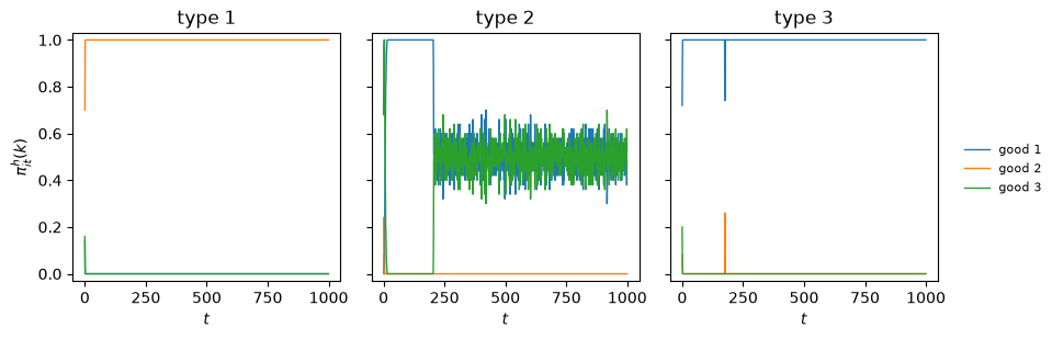
Fig. 95.1 Holdings in Economy A1.1

For roughly the first two hundred periods type 2 agents hold good 1 and nothing else: they have acquired money but do not yet spend it.

The rule that buys good 2 with good 1 has not yet been given a chance, for a reason we explain in Economy A2.1: when theory predicts speculation, and once it wins its first auctions type 2 enters the cycle “acquire money, spend money”.

From then on type 2’s holdings fluctuate, because which good a type 2 agent holds depends on where it is in that cycle.

The next figure shows the trades themselves, averaged over the last hundred periods.

plot_flows(sim_a11)

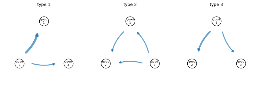
Fig. 95.2 Exchange pattern discovered in Economy A1.1

The fundamental equilibrium triangle is there: type 1 gives up good 2 for good 1, type 3 gives up good 1 for good 3, and type 2 runs both legs, giving up good 3 for good 1 and later good 1 for good 2.

Good 1 circulates as money.

The picture also has arrows that the fundamental equilibrium does not, and they are not thin: type 3 gives up good 1 for good 2 about twice as often as it gives up good 1 for good 3, and type 1 gives up good 2 for good 3 about as often as type 2 runs either of its equilibrium legs.

Each is a payoff-neutral trade of the kind described above, in which the agent eats what it receives and produces its own good again; the partner gains, because type 1 now gets good 1 from type 3 as well as from type 2, and type 2 gets good 2 for its good 3 directly.

The paper’s run had none of these trades, but nothing in the accounting rules them out.

We can also look inside type 1’s classifier systems and read off the rule that wins in each state, first for exchange and then for consumption.

pd.concat([winners(sim_a11, 0), winners(sim_a11, 0, exchange=False)])

	winning rule	strength	times used
state
good 1, good 1	##0 100 -> 1	32.09	22404
good 1, good 2	#0# 0## -> 1	7.93	5
good 1, good 3	#0# 0## -> 1	7.93	5
good 2, good 1	##0 100 -> 1	32.09	22404
good 2, good 2	010 0## -> 1	-0.14	9320
good 2, good 3	010 001 -> 1	-0.10	6370
good 3, good 1	001 #0# -> 1	40.69	2
good 3, good 2	#0# 0## -> 1	7.93	5
good 3, good 3	001 #0# -> 1	40.69	2
good 1	100 -> 1	66.35	22389
good 2	010 -> 1	-0.33	18730
good 3	#0# -> 1	-0.34	6556

The rule that does the work, ##0 100 -> 1, says “if I hold anything but good 3 and my partner holds good 1, trade”: a general rule.

In the state (good 2, good 3) the winning rule accepts good 3, but a type 1 agent who acquires good 3 eats it at once and produces good 2 again, which leaves him exactly where refusing would have.

That is the payoff-neutral trade described above, and it is why we read the outcome from holdings, which never show type 1 holding good 3, rather than from the winning actions.

The paper’s run (its Table 6) had type 1 refusing good 3 instead, which leads to the same holdings.

Is seed 0 typical?

sims_a11 = across_seeds(economy_a11, 1000)
H_a11 = final_holdings(sims_a11)
F_a11 = np.array([trade_rates(sim) for sim in sims_a11])
d, n = distance(H_a11, fundamental), len(sims_a11)
print(f"runs within 0.1 of the fundamental equilibrium: {np.sum(d < 0.1)} of {n}")
print(f"largest distance in any run: {d.max():.3f}")
print(f"runs in which type 3 gives good 1 for good 2:   {np.sum(F_a11[:, 2, 0, 1] > 0.02)} of {n}")
print(f"runs in which type 1 gives good 2 for good 3:   {np.sum(F_a11[:, 0, 1, 2] > 0.02)} of {n}")

runs within 0.1 of the fundamental equilibrium: 20 of 20
largest distance in any run: 0.060
runs in which type 3 gives good 1 for good 2:   17 of 20
runs in which type 1 gives good 2 for good 3:   15 of 20

In every run the holdings settle on the unique stationary equilibrium, and in most runs the payoff-neutral trades appear alongside it.

The medium of exchange is learnable.

95.6. Economy A2.1: when theory predicts speculation

Economy A2 differs from A1 only in that \(u_i = 500\) instead of \(100\).

That is enough to violate the Kiyotaki-Wright inequality (95.4), so for patient agents the unique stationary equilibrium is now the speculative one, in which type 1 agents accept good 3 in the expectation of trading it for good 1.

Do our adaptive agents find it?

economy_a21 = replace(economy_a11, name='A2.1', u=500.0)

sim_a21 = Simulation(economy_a21, seed=0)
sim_a21.run(1000)

speculative = pd.DataFrame([[0, 0.707, 0.293],        # the paper's Table 8b
                            [0.586, 0, 0.414],
                            [1, 0, 0]],
                           index=type_names(economy_a21),
                           columns=good_names(economy_a21))
print("simulated holdings at t = 1000\n", holdings(sim_a21), "\n")
print("speculative equilibrium\n", speculative)

simulated holdings at t = 1000
         good 1  good 2  good 3
type 1   0.000     1.0   0.000
type 2   0.524     0.0   0.476
type 3   1.000     0.0   0.000 

speculative equilibrium
         good 1  good 2  good 3
type 1   0.000   0.707   0.293
type 2   0.586   0.000   0.414
type 3   1.000   0.000   0.000

The answer is no.

The simulated holdings are those of the fundamental pattern: type 1 agents hold good 2 and never good 3, whereas speculation requires them to hold good 3 nearly thirty percent of the time.

Here is what happens across seeds.

sims_a21 = across_seeds(economy_a21, 1000)
H_a21 = final_holdings(sims_a21)
n = len(sims_a21)
print(f"type 1 holds good 3 more than 5% of the time:  {np.sum(H_a21[:, 0, 2] > 0.05)} of {n}")
print(f"within 0.1 of the fundamental pattern:         "
      f"{np.sum(distance(H_a21, fundamental) < 0.1)} of {n}")
print(f"type 2 holds good 1 less than 10% of the time: {np.sum(H_a21[:, 1, 0] < 0.1)} of {n}")
print(f"type 2 holds good 1 more than 90% of the time: {np.sum(H_a21[:, 1, 0] > 0.9)} of {n}")

type 1 holds good 3 more than 5% of the time:  0 of 20
within 0.1 of the fundamental pattern:         10 of 20
type 2 holds good 1 less than 10% of the time: 9 of 20
type 2 holds good 1 more than 90% of the time: 1 of 20

Type 1 never speculates.

Half the runs are near the fundamental pattern at \(t = 1000\).

In nearly all the others type 2 almost never holds good 1: types 2 and 3 have stopped trading with each other, so type 2 never acquires the money it needs to buy good 2.

In one run type 2 holds good 1 all the time: it has money but never spends it, as in the first two hundred periods of our A1.1 run.

Here is the first run of the more common kind, seen through the exchange rules of type 3 agents who hold good 1 and meet a type 2 agent holding good 3.

locked = int(np.flatnonzero(H_a21[:, 1, 0] < 0.1)[0])
sim_locked = sims_a21[locked]
print(f"seed {locked}\n", holdings(sim_locked), "\n")
c = contenders(sim_locked, 2, 0, 2)          # type 3 holds good 1, meets good 3
pd.concat([c.head(2), c[c['rule'] == '100 001 -> 1']])

seed 2
         good 1  good 2  good 3
type 1     0.0     1.0     0.0
type 2     0.0     0.0     1.0
type 3     1.0     0.0     0.0

	rule	strength	times used
0	##0 001 -> 0	0.1	16714
1	100 001 -> 0	0.0	1
2	100 001 -> 1	0.0	0

The type 3 agent wants good 3, which is worth 500 to it, yet the winning rule ##0 001 -> 0 refuses to trade.

Its strength is only \(0.1\), but it is positive, while the specific rule that would trade, 100 001 -> 1, has never been used and still has its initial strength of zero.

The refusal rule earned a large payment in the first periods, when a general consumption rule that also covered good 3 followed it.

With \(1/\tau\) averaging, the average remembers that windfall for thousands of uses.

This is optimistic initialization’s failure mode, and the greedy auction never gives the trade rule a chance until the refusal rule’s average sinks below zero.

That does happen eventually, so runs locked in this way are slow rather than stuck for good.

We continue the runs that were not near the fundamental pattern for another 5,000 periods.

slow = [sim for sim, h in zip(sims_a21, H_a21) if distance(h, fundamental) >= 0.1]
for sim in slow:
    sim.run(5000)
H_slow = final_holdings(slow)
print(f"runs not near the fundamental pattern at t = 1000: {len(slow)}")
print(f"of these, within 0.1 of it at t = 6000:            "
      f"{np.sum(distance(H_slow, fundamental) < 0.1)}")
print(f"of these, type 1 holds good 3 more than 5%:        {np.sum(H_slow[:, 0, 2] > 0.05)}")

runs not near the fundamental pattern at t = 1000: 10
of these, within 0.1 of it at t = 6000:            10
of these, type 1 holds good 3 more than 5%:        0

All of these runs reach the fundamental pattern by \(t = 6000\), and type 1 still never speculates.

Lock-in is more frequent here than in Economy A1.1, plausibly because \(u_1\) is five times larger, and so are the early windfalls that the averages must forget.

Not every lock-in wears off, though.

Other seeds turn up a second failure mode, and seed 24 shows it.

sim_24 = Simulation(economy_a21, seed=24)
sim_24.run(6000)
print(holdings(sim_24), "\n")
winners(sim_24, 1, exchange=False)

        good 1  good 2  good 3
type 1     0.0     1.0     0.0
type 2     0.0     0.0     1.0
type 3     1.0     0.0     0.0

	winning rule	strength	times used
state
good 1	##0 -> 1	146.86	123378
good 2	##0 -> 1	146.86	123378
good 3	001 -> 0	-12.61	175852

This time type 3 does accept good 3; the trouble is with type 2.

It trades good 3 for good 1, as in the fundamental pattern, but then eats the good 1 instead of keeping it to buy good 2 from type 1, so it ends every period holding good 3 again.

The rule responsible is the general consumption rule ##0 -> 1, which says “eat” whether type 2 holds good 1 or good 2.

Eating good 2 is right and earns type 2 its utility of consumption, which keeps the rule’s strength high; eating good 1 is wrong, but the same rule decides that state too.

The specific rule that would keep good 1, 100 -> 0, was tried only a few times and sits far below the general rule’s strength, an average that includes every meal of good 2, so under the argmax auction it never wins again.

So this run is stuck for good: seed 24, and seed 26 in the same way, are still in this pattern at \(t = 24{,}000\).

Optimistic initialization lets a rule that was once lucky shut out an untried rival; this second lock-in is the work of an overgeneral consumption rule, one that earns well in one state and shuts out the specific rule that would act correctly in another.

Type 1 still never speculates: across seeds 20 to 59 it holds good 3 no more than 5 percent of the time in every run.

So the agents do not find A2’s equilibrium.

For patient agents the speculative equilibrium is the unique stationary equilibrium of this economy, so this is not learning selecting among equilibria.

It is convergence to an outcome that is not an equilibrium of the economy the agents live in.

The paper reached the same verdict from a single run, and its diagnosis is worth quoting in full:

Patience requires experience. The transfer system inside the classifier system is designed to converge to a set of long-run average strengths. In the limit, the artificially intelligent agents should behave as long-run average payoff maximizers, since the steady-state strengths weight payoffs by their relative frequencies. It takes time, however, for optimal rules to achieve the desired strengths. The behavior of our artificially intelligent agents can be very myopic at the beginning. In economies, such as Economy A2, in which the nature of the equilibrium changes with the discount rate, this early myopia might have a perverse effect in diverting the economy towards a low discount-factor stationary equilibrium, such as the fundamental equilibrium. The underlying algorithm has to provide enough experimentation to avoid an early ‘lock in’. The present algorithm seems defective in that it has too little experimentation to support the speculative equilibrium even in the long simulations we have run.

The paper’s footnote 14 adds that a fundamental equilibrium exists in A2 only if the discount factor is sufficiently low.

Its footnote 15 reports a telling contrast: in experiments by Marimon and Miller with a genetic algorithm that breeds whole trading strategies (the approach the paper’s footnotes 1 and 3 describe), 25 of 30 runs of Economy A2 converged to the speculative equilibrium.

Their agents had no bucket brigade to credit: each strategy was judged as a whole.

The paper also points to a second culprit.

In its run, type 1’s winning exchange rule accepted good 3 (its Table 9d), but type 1’s winning consumption rules were “too general (have too many # signs) to distinguish among goods stored”, so type 1 ate good 3 rather than carrying it to a type 3 agent.

Accepting good 3 and then eating it is payoff-equivalent to refusing it, which is why the holdings looked fundamental.

Our seed 0 shows the same thing.

pd.concat([winners(sim_a21, 0).loc[['good 2, good 1', 'good 2, good 3']],
           winners(sim_a21, 0, exchange=False).loc[['good 1', 'good 3']]])

	winning rule	strength	times used
state
good 2, good 1	0## ##0 -> 1	96.82	29260
good 2, good 3	010 0## -> 1	0.30	10707
good 1	100 -> 1	334.29	17421
good 3	#0# -> 1	1.08	5983

Type 1’s winning exchange rule in the state (good 2, good 3), 010 0## -> 1, accepts good 3, and the consumption rule that wins when type 1 holds good 3 is the general rule #0# -> 1, “if I do not hold good 2, eat”.

So far this is the paper’s Table 9d.

But generality is not what makes type 1 eat good 3 here.

Here are all of type 1’s consumption rules that match good 3.

c = sim_a21.C
rows = [r for r in range(c.cond.shape[1]) if (c.match[0, r] >> 2) & 1]
pd.DataFrame({'rule': [rule_string(c.cond[0, r], c.action[0, r], 3) for r in rows],
              'strength': c.strength[0, rows].round(2),
              'times used': c.used[0, rows] - 1})

	rule	strength	times used
0	001 -> 0	-11.59	1
1	001 -> 1	-0.48	13
2	0## -> 0	-9.32	6
3	0## -> 1	-0.68	141
4	#0# -> 0	-13.09	5
5	#0# -> 1	1.08	5983

The specific rule that eats good 3 has a strength near zero, while the specific rule that carries it, tried only once, has a strength near \(-12\).

Carrying good 3 costs 20 this period, against 1 for eating it, and the reward for carrying it, a chance to trade it for good 1 next period, reaches the carrying rule only through the bucket brigade, heavily discounted.

Type 1 therefore never carries good 3 into the next period, and the holdings are fundamental.

Three mechanisms are therefore at work in A2:

1. Impatience. Even at rest, the bucket brigade values the future at a tiny discount factor, which the next section derives.

2. Greedy lock-in. The argmax auction stops experimenting once untried rules are used up, as in the trapped runs above.

3. Overconsumption by general consumption rules, which makes accepting good 3 pointless, as in the paper’s Table 9, and in seed 24 keeps type 2 from holding money.

Exercise 95.3, Exercise 95.4 and Exercise 95.5 take them apart one at a time.

95.7. The bucket brigade’s discount factor

The paper hoped that strengths built from long-run averages would make the agents behave like long-run average payoff maximizers once the strengths settled down.

The stationarity conditions say otherwise.

Take an agent whose exchange rule \(e'\) at \(t+1\) follows a consumption rule \(c\) at \(t\), and whose consumption rule \(c'\) at \(t+1\) follows \(e'\).

From the second stationarity condition, \((1 + b_1(e'))S_{e'} = \mathbb{E}[b_2(c') S_{c'}]\).

Substituting it into the first gives

(95.8)\[(1 + b_2(c)) S_c = \mathbb{E}\bigl[U(\gamma_c)\bigr] + \mathbb{E}\Bigl[\beta_{\rm eff}\,(1 + b_2(c')) S_{c'}\Bigr], \qquad \beta_{\rm eff} = \frac{b_1(e')\, b_2(c')}{(1 + b_1(e'))(1 + b_2(c'))} .\]

So the scaled strengths \(V_c = (1 + b_2(c)) S_c\) satisfy a Bellman equation for the agent’s current policy, \(V_c = \mathbb{E}[U] + \mathbb{E}[\beta_{\rm eff} V_{c'}]\), with discount factor \(\beta_{\rm eff}\).

The exchange strengths inherit the ranking: among exchange rules of equal specificity, \(S_e\) is proportional to the expected value of the consumption rule that follows \(e\).

When an offer is refused, \(e'\) pays nothing backward, which lowers the effective discount factor further.

def beta_eff(b1, b2):
    "Effective discount factor of the bucket brigade for bid fractions b1, b2."
    return b1 * b2 / ((1 + b1) * (1 + b2))


b11, b12, b21, b22 = 0.025, 0.025, 0.25, 0.25            # Economy A's bids
β_A = beta_eff(b11 + b12, b21 + b22)                     # fully specific rules
print(f"β_eff with A's bids, specific rules:   {β_A:.4f}")
print(f"β_eff with A's bids, general rules:    {beta_eff(b11 + b12 / 5, b21 + b22 / 3):.4f}")
print(f"β_eff with B.1's bids, specific rules: {beta_eff(0.5, 0.5):.4f}")
print(f"β_eff as both bid fractions approach 1: {beta_eff(1, 1):.4f}")

β_eff with A's bids, specific rules:   0.0159
β_eff with A's bids, general rules:    0.0073
β_eff with B.1's bids, specific rules: 0.1111
β_eff as both bid fractions approach 1: 0.2500

With the paper’s bids the agents behave, at rest, as if they discounted the future at a factor of about \(0.016\) per period, and the most general rules, which bid less, at about \(0.007\).

Because \(b/(1+b) < 1/2\) for any bid fraction below one, \(\beta_{\rm eff}\) can never reach \(1/4\).

The source is the averaging itself: a rule’s own bid enters the average it keeps, so each link of the chain passes back only the fraction \(b/(1+b)\) of the value it receives.

What does an agent with discount factor \(\beta\) do in Economy A?

Redoing the argument behind (95.4) for an agent who discounts each period’s payoffs by \(\beta\), a type 1 agent facing given holdings of the other types prefers to hold good 3 if and only if

\[ s_3 - s_2 < \beta \bigl(\pi^h_3(1) - \pi^h_2(1)\bigr) \tfrac{1}{3} u_1 , \]

so lowering \(\beta\) scales up the threshold for \(u_1\) by \(1/\beta\).

for label, β in [("patient agents, β = 1", 1.0), ("bucket brigade, β = β_eff", β_A)]:
    print(f"{label}: fundamental for u_1 < "
          f"{speculation_threshold(s_A, 1.0, 0.5, β):,.0f}, speculative for u_1 > "
          f"{speculation_threshold(s_A, 1.0, 0.586, β):,.0f}")
print(f"A2's u_1 = 500 supports speculation only if β > "
      f"{speculation_threshold(s_A, 1.0, 0.586) / 500:.3f}")

patient agents, β = 1: fundamental for u_1 < 114, speculative for u_1 > 138
bucket brigade, β = β_eff: fundamental for u_1 < 7,182, speculative for u_1 > 8,674
A2's u_1 = 500 supports speculation only if β > 0.275

For an agent with \(\beta = \beta_{\rm eff}\), A2’s \(u_1 = 500\) is far inside the region where the fundamental pattern is the unique equilibrium.

The figure plots the two thresholds against \(\beta\).

βs = np.logspace(-2.5, 0, 200)
fig, ax = plt.subplots(figsize=(7, 4))
ax.loglog(βs, speculation_threshold(s_A, 1.0, 0.5, βs),
          label="fundamental equilibrium exists below")
ax.loglog(βs, speculation_threshold(s_A, 1.0, 0.586, βs), '--',
          label="speculative equilibrium exists above")
for u, name in [(100, "A1"), (500, "A2")]:
    ax.axhline(u, color='k', lw=0.6)
    ax.annotate(f"{name}: $u_1 = {u}$", (βs[0], u * 1.1), fontsize=9)
ax.axvline(β_A, color='C3', lw=1)
ax.axvline(0.25, color='C3', lw=1, ls=':')
ax.annotate(r"$\beta_{\rm eff}$", (β_A * 1.08, 150), color='C3')
ax.annotate("1/4", (0.25 * 1.08, 150), color='C3')
ax.set_xlabel(r"discount factor $\beta$")
ax.set_ylabel(r"$u_1$")
ax.legend(frameon=False, loc='upper right')
plt.show()

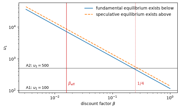
Fig. 95.3 Speculation thresholds for \(u_1\) against the discount factor

Economy A2 supports speculation only for \(\beta\) above \(0.275\), beyond the reach of any bid fractions, so at rest the bucket brigade cannot support A2’s equilibrium with fully specific rules, whatever its bids.

This sharpens the paper’s diagnosis.

Early myopia is real, but it is not only early: the stationary strengths themselves are impatient.

The fundamental pattern – accept a good only if you eat it or it is cheaper to store – is exactly what an impatient agent does, which is the paper’s “low discount-factor stationary equilibrium”.

The same is true of the patterns the classifier systems find in every other economy of this lecture: the fundamental equilibrium of Economy B, the acceptance of fiat money in Economy C (fiat costs nothing to store), and the “lower storage cost” pattern the paper reports for Economy D.

Equation (95.8) is a familiar object.

The scaled strengths are evaluated like the temporal-difference value estimates of reinforcement learning [Sutton and Barto, 2018], which Job Search X: Search with Q-Learning and Inventory Management via Q-Learning apply to a job seeker and to a firm.

The difference is that here the discount factor is not chosen to match the agent’s preferences: it is a by-product of the bid fractions.

The bucket brigade finds the same factor \(b/(1+b)\) per link in a two-link chain, and shows that Holland’s cumulative balances, which do not average, pass a payoff back undiminished but need not converge.

One recursion, many learners explains why, with \(1/\tau\) averaging, the rest points of (95.6)-(95.7) are the objects to study.

Exercise 95.5 checks the threshold by simulation.

95.8. Economy B.1: selecting between two equilibria

Economy B changes the production pattern – type 1 produces good 3, type 2 produces good 1, type 3 produces good 2 – and compresses storage costs to \(s = (1, 4, 9)\), with \(u_i = 100\).

Now there are two stationary equilibria for patient agents: in the fundamental one goods 1 and 2 serve as media of exchange, and in the speculative one goods 2 and 3 do.

B.1 also uses exchange bids ten times A’s, \(b_{11} = b_{12} = 0.25\), as in the paper’s Table 12, which raises \(\beta_{\rm eff}\) to about \(0.11\).

economy_b1 = Economy(
    name='B.1',
    produces=np.array([2, 0, 1]),               # type 1 -> good 3, type 2 -> good 1, ...
    storage_costs=np.array([1.0, 4.0, 9.0]),
    u=100.0,
    b_trade=(0.25, 0.25),
)

sim_b1 = Simulation(economy_b1, seed=0)
sim_b1.run(1000)

fundamental_b = np.array([[0, 0.293, 0.707],    # the paper's Table 10b
                          [1, 0, 0],
                          [0.586, 0.414, 0]])
speculative_b = np.array([[0, 0.586, 0.414],    # the paper's Table 11b
                          [0.707, 0, 0.293],
                          [0, 1, 0]])
paper_b1 = np.array([[0.0, 0.28, 0.72],         # the paper's Table 12b, t = 1000
                     [0.994, 0.0, 0.006],
                     [0.526, 0.474, 0.0]])

print("holdings at t = 500\n", holdings(sim_b1, t=500), "\n")
print("holdings at t = 1000\n", holdings(sim_b1), "\n")
h = holdings(sim_b1).to_numpy()
for name, target in [("fundamental equilibrium", fundamental_b),
                     ("speculative equilibrium", speculative_b),
                     ("paper's table", paper_b1)]:
    print(f"max |simulated - {name}| = {distance(h, target):.3f}")
print(f"max |paper's table - fundamental equilibrium| = "
      f"{distance(paper_b1, fundamental_b):.3f}")

holdings at t = 500
         good 1  good 2  good 3
type 1    0.00   0.292   0.708
type 2    1.00   0.000   0.000
type 3    0.57   0.430   0.000 

holdings at t = 1000
         good 1  good 2  good 3
type 1   0.000   0.266   0.734
type 2   1.000   0.000   0.000
type 3   0.556   0.444   0.000 

max |simulated - fundamental equilibrium| = 0.030
max |simulated - speculative equilibrium| = 0.556
max |simulated - paper's table| = 0.030
max |paper's table - fundamental equilibrium| = 0.060

The run ends near the fundamental equilibrium of Economy B, closer to it than the paper’s own run.

plot_holdings(sim_b1)

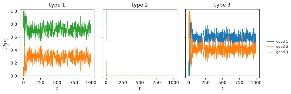
Fig. 95.4 Holdings in Economy B.1

Across seeds:

H_b1 = final_holdings(across_seeds(economy_b1, 1000))
d_f, d_s = distance(H_b1, fundamental_b), distance(H_b1, speculative_b)
print(f"within 0.1 of the fundamental equilibrium: {np.sum(d_f < 0.1)} of {len(H_b1)}")
print(f"within 0.1 of the speculative equilibrium: {np.sum(d_s < 0.1)} of {len(H_b1)}")
print(f"smallest distance from the speculative equilibrium: {d_s.min():.2f}")
print("holdings in the runs farther than 0.1 from the fundamental equilibrium:")
print(H_b1[d_f >= 0.1].round(2))

within 0.1 of the fundamental equilibrium: 18 of 20
within 0.1 of the speculative equilibrium: 0 of 20
smallest distance from the speculative equilibrium: 0.29
holdings in the runs farther than 0.1 from the fundamental equilibrium:
[[[0.   0.49 0.51]
  [1.   0.   0.  ]
  [0.   1.   0.  ]]

 [[0.   0.27 0.73]
  [1.   0.   0.  ]
  [0.47 0.53 0.  ]]]

In 18 of the 20 runs the holdings end within 0.1 of the fundamental equilibrium, and no run comes within 0.29 of the speculative one.

Of the other two runs, one is just outside the 0.1 band, and in the other type 3 agents never trade their good 2 for good 1.

Here learning does select between two equilibria, and it selects the fundamental one.

The paper reports one more feature that our run does not reproduce: at \(t = 500\) its B.1 looked speculative, and only by \(t = 1000\) had it “practically converged to the fundamental equilibrium”.

The paper read that movement as evidence that the selection was not “the result of myopic behavior”.

In our run there is no speculative phase beyond the first few periods, which are dominated by the random initial holdings, so the movement is not something we can confirm.

And The bucket brigade’s discount factor suggests a different reading: the fundamental equilibrium of Economy B is also the one an impatient agent plays, and the bucket brigade is impatient at rest, not just early on.

95.9. The genetic algorithm

Complete enumeration is feasible only because the Kiyotaki-Wright state space is tiny.

In larger problems an agent must work with a limited population of rules that is continually revised.

The paper starts such agents from randomly generated rules and adds four operators: the three we have already met inside the auction, and generalization, a genetic algorithm.

Generalization is called with probability \(f_g(t) = 1/(2\sqrt{t})\) in period \(t\).

When it is called, it works as follows (the paper’s Section 6 and Table 7):

• Potential exterminants are rules that are both weak and seldom used: strength below \(\bar S = 0\) and a counter below \(p_3 = 0.2\) times the largest counter.

• Potential parents are a fraction \(p_2 = 0.7\) of the rules, chosen randomly “in accordance with strength and frequency”; we draw them with probabilities proportional to their counters and then select pairs within them by a roulette wheel on strength.

• Pairs mate until a fraction \(p_1 = 0.2\) of the population has been replaced.

• Generalizing crossover (the paper’s Fig. 4): the pair draws two cut points and focuses on the positions inside them, or, with probability one half, outside them; wherever the parents carry different specific bits in the focus, both children get a \(\#\). Children therefore match everything their parents matched, and more.

• Each child gets the average of its parents’ strengths and replaces the potential exterminant it most resembles, by crowding: \(N = 8\) times (4 for consumption rules) a sample of half the potential exterminants is drawn, the weakest member of each sample is scored by the number of positions it shares with the child plus one if its action differs, and the highest score loses its place.

The paper’s footnote 12 says that more standard Holland algorithms “were first tried without much success, prompting us to produce the modified algorithm described in section 6”.

We therefore use the generalizing crossover in every economy with random rules, and, since the paper’s Table 7 lists no mutation rate, no mutation.

Where the paper is silent we have made the following choices:

• ties in the auction are broken at random;

• generalization is drawn independently for each type’s exchange and consumption systems;

• new rules, including children, start with a counter of 1, so after their first experience the strength they were born with survives only through the bid they paid out of it;

• creation gives the new rule strength zero;

• “weakness” outside the genetic algorithm is the score in weakest;

• specialization, when switched on in a period, applies to every auction in that period;

• each agent’s own decisions form a bucket-brigade chain, as discussed above;

• the goods of Economy D get a five-position one-hot code.

@njit
def roulette(w, rng):
    "Draw an index with probability proportional to the nonnegative weights w."
    x = rng.random() * w.sum()
    for k in range(w.shape[0]):
        x -= w[k]
        if x <= 0:
            return k
    return w.shape[0] - 1


@njit
def generalize(R, i, n_goods, rng, stamp, n_crowd,
               p1=0.2, p2=0.7, p3=0.2, p4=0.5, S_bar=0.0):
    "One call of the paper's genetic algorithm on the classifier system of type i."
    cond, action, S, used = R.cond[i], R.action[i], R.strength[i], R.used[i]
    n, L = cond.shape

    # potential exterminants: weak *and* seldom used
    doomed = [r for r in range(n) if S[r] < S_bar and used[r] < p3 * used.max()]
    if len(doomed) == 0:
        return

    # potential parents: p2 * n rules drawn without replacement, weighted by use
    w = used.astype(np.float64)
    parents = np.zeros(int(p2 * n), np.int64)
    for k in range(parents.shape[0]):
        parents[k] = roulette(w, rng)
        w[parents[k]] = 0.0
    fitness = S[parents] - S[parents].min() + 1e-6

    for _ in range(max(1, int(p1 * n) // 2)):
        mum = parents[roulette(fitness, rng)]
        dad = parents[roulette(fitness, rng)]
        kids = (cond[mum].copy(), cond[dad].copy())

        # generalizing crossover
        cuts = np.sort(rng.integers(0, L + 1, size=2))
        inside = rng.random() < 0.5
        for j in range(L):
            if ((cuts[0] <= j < cuts[1]) == inside and kids[0][j] != WILD
                    and kids[1][j] != WILD and kids[0][j] != kids[1][j]):
                kids[0][j] = WILD
                kids[1][j] = WILD
        strength = 0.5 * (S[mum] + S[dad])

        # crowding: each child replaces the potential exterminant it most resembles
        for kid, act in ((kids[0], action[mum]), (kids[1], action[dad])):
            if len(doomed) == 0:
                return
            size = max(1, int(p4 * len(doomed)))
            victim, best = doomed[0], -1
            for _ in range(n_crowd):
                sample = rng.permutation(len(doomed))[:size]
                cand = doomed[sample[0]]
                for q in sample:
                    if S[doomed[q]] < S[cand]:
                        cand = doomed[q]
                likeness = np.sum(kid == cond[cand]) + (act != action[cand])
                if likeness > best:
                    victim, best = cand, likeness
            set_rule(R, i, victim, kid, act, strength, n_goods, stamp)
            doomed.remove(victim)

95.10. Economy A1.2: learning from random rules

Economy A1.2 has the same parameters as A1.1, but agents begin with 72 exchange rules and 12 consumption rules drawn at random from the 1,458 and 54 possible strings.

Most of these rules are nonsense, and there is no guarantee that the population contains the rules needed to support an equilibrium.

The operators must manufacture them.

economy_a12 = replace(economy_a11, name='A1.2', random_rules=True)

sim_a12 = Simulation(economy_a12, seed=0)
sim_a12.run(2000)

paper_a12 = np.array([[0.0, 0.98, 0.02],        # the paper's Table 7b, t = 2000
                      [0.318, 0.0, 0.682],
                      [1.0, 0.0, 0.0]])
print("holdings at t = 1000\n", holdings(sim_a12, t=1000), "\n")
print("holdings at t = 2000\n", holdings(sim_a12), "\n")
print("paper's table at t = 2000\n", paper_a12, "\n")
print(f"max |paper's table - fundamental equilibrium| = "
      f"{distance(paper_a12, fundamental):.3f}")

holdings at t = 1000
         good 1  good 2  good 3
type 1   0.000   0.942   0.058
type 2   0.424   0.000   0.576
type 3   0.842   0.158   0.000 

holdings at t = 2000
         good 1  good 2  good 3
type 1   0.000   0.946   0.054
type 2   0.422   0.000   0.578
type 3   0.788   0.212   0.000 

paper's table at t = 2000
 [[0.    0.98  0.02 ]
 [0.318 0.    0.682]
 [1.    0.    0.   ]] 

max |paper's table - fundamental equilibrium| = 0.182

Here are the time paths.

plot_holdings(sim_a12)

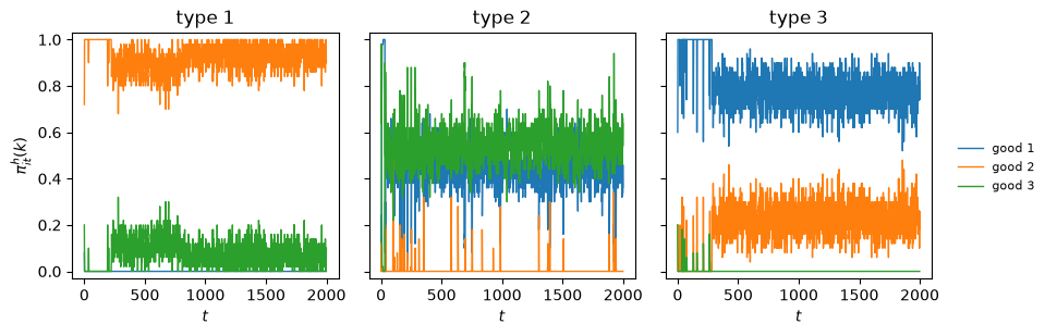
Fig. 95.5 Holdings in Economy A1.2

The fundamental pattern emerges again, though less cleanly than under complete enumeration.

Type 1 mostly holds good 2, type 2 holds only goods 1 and 3, and type 3 mostly holds good 1.

But types 1 and 3 also hold goods that the fundamental equilibrium excludes: in this run type 1 holds good 3 about 5 percent of the time and type 3 holds good 2 about a fifth of the time.

The paper’s run was cleaner for types 1 and 3 but not for type 2: at \(t = 2000\) its type 2 agents held good 1 only 32 percent of the time, and its Table 7e shows type 2 eating good 1 – its money – with probability 0.45 at \(t = 1000\) and 0.23 at \(t = 2000\).

The paper calls this overeating “a minor problem in several of our economies”, associated with states the classifier system visits too rarely to learn about.

Here are the eating frequencies over the last 200 periods of our run.

eating_rates(sim_a12)

	good 1	good 2	good 3
type 1	1.00	0.50	0.53
type 2	0.02	0.98	0.97
type 3	0.56	0.46	1.00

In this run type 2 hardly ever eats its money, which is why its holdings are close to the equilibrium’s even split.

Types 1 and 3 eat “wrong” goods about half the time, which costs them nothing when the good is their own production good (good 2 for type 1, good 1 for type 3).

But type 1 also carries good 3 into the next period about half the times it gets it, at a cost of 20 rather than 1, and type 3 carries good 2 about half the time: these are the rarely visited states the paper blames.

Across seeds:

sims_a12 = across_seeds(economy_a12, 2000)
H_a12 = final_holdings(sims_a12)
eat_money = np.array([eating_rates(sim).iloc[1, 0] for sim in sims_a12])
n = len(H_a12)
print(f"type 1 holds good 2 at least 90% of the time: {np.sum(H_a12[:, 0, 1] >= 0.9)} of {n}")
print(f"type 3 holds good 1 at least 90% of the time: {np.sum(H_a12[:, 2, 0] >= 0.9)} of {n}")
print(f"type 2 holds only goods 1 and 3:              {np.sum(H_a12[:, 1, 1] < 0.05)} of {n}")
print(f"type 2's share of good 1: median {np.median(H_a12[:, 1, 0]):.2f}, "
      f"range {H_a12[:, 1, 0].min():.2f} to {H_a12[:, 1, 0].max():.2f}")
print(f"within 0.1 of the fundamental equilibrium:    "
      f"{np.sum(distance(H_a12, fundamental) < 0.1)} of {n}")
print(f"type 2 eats good 1 at least 40% of the time:  {np.sum(eat_money >= 0.4)} of {n}")

type 1 holds good 2 at least 90% of the time: 16 of 20
type 3 holds good 1 at least 90% of the time: 13 of 20
type 2 holds only goods 1 and 3:              20 of 20
type 2's share of good 1: median 0.19, range 0.09 to 0.50
within 0.1 of the fundamental equilibrium:    5 of 20
type 2 eats good 1 at least 40% of the time:  11 of 20

Seed 0 is one of the better runs.

In every run type 2 holds only goods 1 and 3, and in most runs types 1 and 3 hold their equilibrium goods at least 90 percent of the time.

But type 2’s median share of good 1 is only 0.19, and in about half the runs type 2 eats good 1 at least 40 percent of the time, the overeating of the paper’s run.

Only a quarter of the runs end within 0.1 of the fundamental equilibrium; the paper’s own run was 0.18 away.

General rules survive the genetic algorithm.

share = lambda R: np.mean(R.cond == WILD)
print(f"share of # in exchange rules:    {share(sim_a12.E):.2f}")
print(f"share of # in consumption rules: {share(sim_a12.C):.2f}")

share of # in exchange rules:    0.32
share of # in consumption rules: 0.16

A random string has a \(\#\) in a third of its positions, and generalizing crossover keeps adding them while specialization slowly removes them.

95.11. Economy C: fiat money

Now add a fourth object, fiat money, which the paper calls good 0.

It

• costs nothing to store, \(s_0 = 0\);

• yields no utility to anybody; and

• cannot be consumed.

It is intrinsically worthless.

It is introduced by handing 48 units of it to 48 randomly chosen agents at \(t = 0\), and commodity storage costs are raised to \(s = (9, 14, 29)\) so that no commodity is nearly as cheap to store as money.

The paper’s footnote 17 reports that a version with Economy A’s storage costs did not converge, “probably because the low cost of storing good 1 (0.1) made this good too good a substitute for fiat money”.

Agents start from 150 random exchange rules and 20 random consumption rules each, out of 13,122 and 162 possible strings.

economy_c = Economy(
    name='C',
    produces=np.array([1, 2, 0]),
    storage_costs=np.array([9.0, 14.0, 29.0, 0.0]),    # fiat money is the last good
    u=100.0,
    random_rules=True,
    n_trade_rules=150,
    n_consume_rules=20,
    b_consume=(0.025, 0.25),
    n_fiat=48,
)

sim_c = Simulation(economy_c, seed=0)
sim_c.run(2000)

fundamental_c = np.array([[0, 0.74, 0, 0.26],       # the paper's Table 14b
                          [0.26, 0, 0.42, 0.32],
                          [0.62, 0, 0, 0.38]])
paper_c = np.array([[0, 0.54, 0, 0.46],             # the paper's Table 15b, t = 1250
                    [0.18, 0, 0.53, 0.28],
                    [0.77, 0.01, 0, 0.21]])
print("holdings at t = 750\n", holdings(sim_c, t=750), "\n")
print("holdings at t = 1250\n", holdings(sim_c, t=1250), "\n")
h = holdings(sim_c, t=1250).to_numpy()
print(f"max |simulated - fundamental equilibrium| = {distance(h, fundamental_c):.3f}")
print(f"max |simulated - paper's table|           = {distance(h, paper_c):.3f}")

holdings at t = 750
         good 1  good 2  good 3   fiat
type 1   0.000   0.676   0.042  0.282
type 2   0.108   0.000   0.588  0.304
type 3   0.626   0.000   0.000  0.374 

holdings at t = 1250
         good 1  good 2  good 3   fiat
type 1   0.000   0.628   0.070  0.302
type 2   0.096   0.000   0.538  0.366
type 3   0.708   0.000   0.000  0.292 

max |simulated - fundamental equilibrium| = 0.164
max |simulated - paper's table|           = 0.158

Every type holds fiat money roughly 30 percent of the time, close to the theoretical fundamental equilibrium (the paper’s Table 14b); the paper’s own run (its Table 15b) has type 1 holding fiat money more often, 46 percent of the time.

The largest discrepancy from the theory is type 2’s holding of good 1, about 0.10 in our run against 0.26 in theory and 0.18 in the paper’s run: our type 2 agents rely on fiat money rather than good 1 as their medium of exchange more than the theory says.

plot_holdings(sim_c)

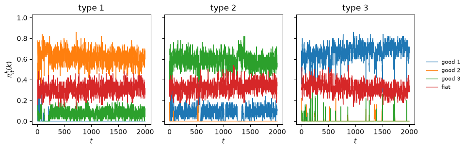
Fig. 95.6 Holdings in Economy C

The exchange pattern shows money changing hands.

plot_flows(sim_c)

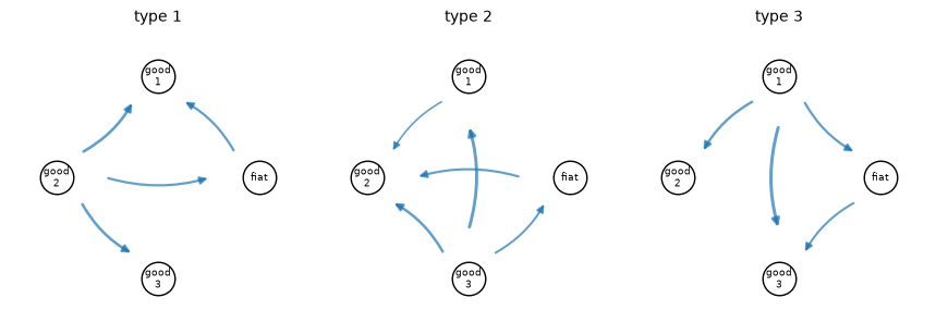
Fig. 95.7 Exchange pattern discovered in Economy C

The arrows into and out of the fiat node show money changing hands in both directions for every type: agents give up their production good to acquire it, and give it up to acquire the good they consume.

Good 1 still serves as a second money for type 2, which gives up good 3 for good 1 and good 1 for good 2.

The payoff-neutral trades of Economy A1.1 appear again: type 1 gives up good 2 for good 3, and type 3 gives up good 1 for good 2.

Across seeds:

H_c = final_holdings(across_seeds(economy_c, 1250))
n = len(H_c)
print(f"every type holds fiat at least 10% of the time: "
      f"{np.sum(H_c[:, :, 3].min(axis=1) >= 0.1)} of {n}")
print("holdings averaged over runs:")
print(pd.DataFrame(H_c.mean(axis=0), index=type_names(economy_c),
                   columns=good_names(economy_c)).round(2))
print(f"within 0.1 of the fundamental equilibrium:      "
      f"{np.sum(distance(H_c, fundamental_c) < 0.1)} of {n}")
print(f"within 0.2 of the fundamental equilibrium:      "
      f"{np.sum(distance(H_c, fundamental_c) < 0.2)} of {n}")
print("holdings in runs where some type holds fiat less than 10% of the time:")
print(H_c[H_c[:, :, 3].min(axis=1) < 0.1].round(2))

every type holds fiat at least 10% of the time: 18 of 20
holdings averaged over runs:
        good 1  good 2  good 3  fiat
type 1    0.00    0.60    0.05  0.35
type 2    0.16    0.00    0.54  0.30
type 3    0.63    0.06    0.00  0.31
within 0.1 of the fundamental equilibrium:      2 of 20
within 0.2 of the fundamental equilibrium:      14 of 20
holdings in runs where some type holds fiat less than 10% of the time:
[[[0.   0.04 0.   0.96]
  [0.96 0.   0.04 0.  ]
  [0.98 0.01 0.01 0.  ]]

 [[0.   0.49 0.   0.51]
  [0.17 0.06 0.67 0.1 ]
  [0.52 0.13 0.   0.36]]]

In 18 of the 20 runs every type holds fiat money at least 10 percent of the time.

In one of the other two, type 1 agents hoard fiat money while types 2 and 3 hold almost none; in the other, type 2’s share of fiat money is just under 10 percent.

On average across runs the holdings are within about 0.15 of the theoretical equilibrium: type 1 holds more fiat money and less good 2 than in theory, and type 2 less good 1 and more good 3, as in seed 0.

Those gaps are why only 2 runs come within 0.1 of the equilibrium, while 14 come within 0.2.

Nothing in the environment told the agents to do this.

Each agent discovered only that rules which end up holding the costless object earn more than rules that do not, and, because everyone was discovering this at once, the belief became self-confirming.

The discovery asks little of the agents: fiat money is the cheapest object to store, so even an impatient agent accepts it, provided others will take it in turn.

95.12. Economy D: five goods, five types

The last economy has five types and five goods, with production

type \(i\)	produces	consumes
1	good 3	good 1
2	good 4	good 2
3	good 5	good 3
4	good 1	good 4
5	good 2	good 5

storage costs \(s = (1, 4, 9, 20, 30)\) from the paper’s Table 4, and \(u_i = 200\).

Each agent carries 180 exchange rules and 20 consumption rules.

The authors emphasize that they had no analytical characterization of equilibrium for this economy, and used the simulation to suggest what an equilibrium might look like.

economy_d = Economy(
    name='D',
    produces=np.array([2, 3, 4, 0, 1]),         # type 1 -> good 3, type 2 -> good 4, ...
    storage_costs=np.array([1.0, 4.0, 9.0, 20.0, 30.0]),
    u=200.0,
    random_rules=True,
    n_trade_rules=180,
    n_consume_rules=20,
)

sim_d = Simulation(economy_d, seed=0)
sim_d.run(2000)
holdings(sim_d)

	good 1	good 2	good 3	good 4	good 5
type 1	0.000	0.114	0.886	0.000	0.000
type 2	0.032	0.000	0.112	0.814	0.042
type 3	0.046	0.052	0.000	0.028	0.874
type 4	0.832	0.018	0.094	0.000	0.056
type 5	0.208	0.546	0.246	0.000	0.000

The time paths show how the holdings got there.

plot_holdings(sim_d)

Fig. 95.8 Holdings in Economy D

Two features stand out.

First, the diagonal is zero: no type ends a period holding the good it consumes, because it eats it.

Second, every type holds mostly the good it produces; at the end of this run only type 5 holds other goods much of the time, and type 1 holds the cheaper good 2 about a tenth of the time.

The time paths have not fully settled; type 2’s holdings in particular swing between goods 4 and 1 for much of the run.

The paper’s run looks different in its details: at \(t = 1750\) its type 1 agents held the cheaper good 2 83 percent of the time, and its type 3 agents split their holdings between good 2 and good 5.

Let us classify the trades that actually take place by what the agent acquires.

def trade_composition(sim, window=200):
    """
    Shares of realized trades in which the agent acquires its own consumption
    good, a good cheaper to store than the one given up, or neither; and the
    share of 'neither' trades that give up the agent's own production good
    and are then eaten (payoff-neutral).
    """
    econ = sim.econ
    f = np.array(sim.exch_hist)[-window:].sum(axis=0)
    c = np.array(sim.cons_hist[-window:]).sum(axis=0)
    eat = c[:, :, 1] / np.maximum(c[:, :, 0], 1)
    s = econ.storage_costs
    out = {'own consumption good': 0.0, 'a cheaper good': 0.0, 'neither': 0.0}
    neutral = 0.0
    for i in range(econ.n_types):
        for j in range(econ.n_goods):
            for k in range(econ.n_goods):
                if j == k:
                    continue
                key = ('own consumption good' if k == i else
                       'a cheaper good' if s[k] < s[j] else 'neither')
                out[key] += f[i, j, k]
                if key == 'neither' and j == econ.produces[i]:
                    neutral += f[i, j, k] * eat[i, k]
    total = sum(out.values())
    out = {k: v / total for k, v in out.items()}
    out['  of which payoff-neutral'] = neutral / total
    return pd.Series(out, name='share of realized trades').round(3)


trade_composition(sim_d)

own consumption good         0.339
a cheaper good               0.307
neither                      0.354
  of which payoff-neutral    0.183
Name: share of realized trades, dtype: float64

About two thirds of realized trades acquire either the agent’s own consumption good or a good that is cheaper to store, which is the pattern the paper describes.

About half of the remaining third are payoff-neutral: the agent gives up its own production good for a dearer good, eats it, and produces its own good again.

The rest, about a sixth of all trades, fit neither description.

Here are the same statistics for ten seeds, together with the number of times per period an agent of each type eats its own good.

sims_d = across_seeds(economy_d, 2000, seeds=range(10))
comp = pd.DataFrame([trade_composition(sim) for sim in sims_d])
print(comp.describe().loc[['mean', 'min', 'max']].round(2), "\n")
own = np.array([[np.array(sim.cons_hist[-200:]).sum(axis=0)[i, i, 1] / (200 * 50)
                 for i in range(5)] for sim in sims_d])
print("own-good consumption per agent per period, smallest over runs:",
      own.min(axis=0).round(3))

      own consumption good  a cheaper good  neither    of which payoff-neutral
mean                  0.33            0.31     0.37                       0.18
min                   0.29            0.28     0.33                       0.15
max                   0.38            0.34     0.40                       0.23 

own-good consumption per agent per period, smallest over runs: [0.04  0.1   0.041 0.059 0.07 ]

The shares change little from run to run, and every type eats its own good in every run.

The paper summarizes its own run this way:

From the simulation results, we can see that the trading patterns nearly seem to describe a fundamental equilibrium in which agents are only willing to trade for commodities of lower cost than the one currently in storage, except that they always accept the commodity of their type. Some speculative moves can be detected.

Our runs share the first part of that description, with two qualifications: a third of the trades fit neither pattern, half of them because the “consume anything” rule makes them payoff-neutral, and in our displayed run the holdings have not settled down.

The paper’s example of a speculative move – type 2 agents accepting good 3 from type 1 in exchange for good 1, in order to trade it to type 3 for good 2 – comes from its own run.

What the simulation delivers is a candidate pattern of trade, which would still have to be checked against the equilibrium conditions, as the authors note.

95.13. Concluding remarks

Marimon, McGrattan and Sargent’s agents know very little.

They do not know their own utility functions, they do not know storage costs, they do not know the distribution of goods across the population, and they certainly do not solve dynamic programs.

They recognize utility when they experience it and costs when they bear them, and they keep running averages.

Out of this the following emerges.

• A medium of exchange is learnable. With a complete list of rules, Economy A1 reaches its unique stationary equilibrium in every run; from random rules the agents get most of the way, overeating money as the paper’s agents did.

• Selection, and its limits. In Economy B, with two equilibria, the classifier systems select the fundamental one in most runs and the speculative one in none. In Economy A2, whose only equilibrium for patient agents is speculative, they never speculate: most runs converge, sometimes very slowly, to an outcome that is not an equilibrium of that economy, and a few lock into a pattern with even less trade.

• Why: the agents are impatient. At stationary strengths the bucket brigade values the future with a discount factor \(b_1 b_2/((1+b_1)(1+b_2))\), about \(0.016\) with the paper’s bids and below \(1/4\) for any bids, and the patterns the agents find are those of impatient agents. The greedy auction and overgeneral consumption rules add to the effect.

• Institutions can be discovered. In nearly every run, Economy C’s agents built a fiat monetary system out of nothing but their own experience of storage costs.

• The method proposes candidates. Economy D produced a pattern of trade in a model its authors had not solved, though not one that has been verified to be an equilibrium.

The paper is candid about what is missing.

There are no convergence theorems, only a sketch of how stochastic approximation arguments might supply them, and the authors judge their algorithm to provide “too little experimentation”.

Experimentation is part of the story, but the stationary strengths show that more of it would not be enough: an agent built this way values a payoff one period ahead at less than a quarter of its worth, whatever its bids.

1993 Prospects for Bounded Rationality in Macroeconomics takes stock of what the series has delivered, and enters Economy A2 on the debit side of the ledger.

95.14. Exercises

Exercise 95.1

Economy A2.2 is Economy A2 – with \(u_i = 500\) – but started from randomly generated rules and evolved with the genetic algorithm, exactly as A1.2 relates to A1.1.

The paper’s summary table lists its equilibrium type as speculative, and the authors report that after 1000 iterations the economy had not converged, with trading patterns closer to the fundamental equilibrium than to the speculative one in period 1000 – “(The reverse was true in period 500.)”

Simulate it for 2000 periods and report holdings at \(t = 500\), \(t = 1000\) and \(t = 2000\).

Then repeat for 20 seeds.

Does the extra experimentation supplied by the genetic algorithm produce speculation at any of these dates?

Solution

economy_a22 = replace(economy_a21, name='A2.2', random_rules=True)

sim_a22 = Simulation(economy_a22, seed=0)
sim_a22.run(2000)
for t in (500, 1000, 2000):
    print(f"t = {t}\n", holdings(sim_a22, t=t), "\n")

t = 500
         good 1  good 2  good 3
type 1   0.000   1.000   0.000
type 2   0.438   0.000   0.562
type 3   0.788   0.212   0.000 

t = 1000
         good 1  good 2  good 3
type 1   0.000   1.000   0.000
type 2   0.428   0.000   0.572
type 3   0.722   0.278   0.000 

t = 2000
         good 1  good 2  good 3
type 1   0.000   1.000   0.000
type 2   0.404   0.000   0.596
type 3   0.732   0.268   0.000

Now the same experiment for 20 seeds, recording holdings at each date.

sims_a22 = across_seeds(economy_a22, 2000)
for t in (500, 1000, 2000):
    H = final_holdings(sims_a22, t)
    closer = distance(H, speculative.to_numpy()) < distance(H, fundamental)
    print(f"t = {t}: type 1 holds good 3 > 5% in {np.sum(H[:, 0, 2] > 0.05)} runs "
          f"(at most {H[:, 0, 2].max():.2f} of the time); closer to speculative "
          f"than to fundamental in {np.sum(closer)} runs")

t = 500: type 1 holds good 3 > 5% in 2 runs (at most 0.16 of the time); closer to speculative than to fundamental in 0 runs
t = 1000: type 1 holds good 3 > 5% in 1 runs (at most 0.12 of the time); closer to speculative than to fundamental in 0 runs
t = 2000: type 1 holds good 3 > 5% in 3 runs (at most 0.15 of the time); closer to speculative than to fundamental in 1 runs

No.

In this run type 1 never holds good 3 at any of the three dates.

Across 20 runs, at each date type 1 holds good 3 more than 5 percent of the time in at most three runs, and never as often as the speculative equilibrium’s 29 percent.

Only one run, at \(t = 2000\), is even marginally closer to the speculative holdings than to the fundamental ones, and our runs do not reproduce the paper’s report that its run looked more speculative at \(t = 500\).

Randomizing the initial rules and adding the genetic algorithm can manufacture rules that accept good 3, but it does not change the discount factor at which the bucket brigade values holding it (The bucket brigade’s discount factor).

Exercise 95.2

Economy B.2 is Economy B started from random rules, with the genetic algorithm and A’s bids.

The paper reports that it “had not converged after 2000 periods” but was “moving towards the fundamental equilibrium”, with holdings at \(t = 2000\) of \((0, 0.354, 0.646)\) for type 1, \((0.996, 0, 0.004)\) for type 2 and \((0.268, 0.732, 0)\) for type 3.

Simulate it, compare its holdings with the two equilibria of Economy B and with the paper’s run, and compare its distance from the fundamental equilibrium with B.1’s across 20 seeds.

Solution

economy_b2 = replace(economy_b1, name='B.2', random_rules=True,
                     b_trade=(0.025, 0.025))
sim_b2 = Simulation(economy_b2, seed=0)
sim_b2.run(2000)

paper_b2 = np.array([[0, 0.354, 0.646], [0.996, 0, 0.004], [0.268, 0.732, 0]])
rows = {'B.2 simulated, t = 2000': holdings(sim_b2).to_numpy(),
        'fundamental equilibrium': fundamental_b,
        'speculative equilibrium': speculative_b,
        "paper's B.2, t = 2000": paper_b2}
pd.concat({k: pd.DataFrame(v, index=type_names(economy_b2),
                           columns=good_names(economy_b2)).round(3)
           for k, v in rows.items()})

		good 1	good 2	good 3
B.2 simulated, t = 2000	type 1	0.000	0.100	0.900
	type 2	0.856	0.000	0.144
	type 3	0.112	0.888	0.000
fundamental equilibrium	type 1	0.000	0.293	0.707
	type 2	1.000	0.000	0.000
	type 3	0.586	0.414	0.000
speculative equilibrium	type 1	0.000	0.586	0.414
	type 2	0.707	0.000	0.293
	type 3	0.000	1.000	0.000
paper's B.2, t = 2000	type 1	0.000	0.354	0.646
	type 2	0.996	0.000	0.004
	type 3	0.268	0.732	0.000

Now compare B.2 with B.1 across seeds.

H_b2 = final_holdings(across_seeds(economy_b2, 2000))
for name, H in [("B.1", H_b1), ("B.2", H_b2)]:
    print(f"{name}: median distance to fundamental "
          f"{np.median(distance(H, fundamental_b)):.2f}, to speculative "
          f"{np.median(distance(H, speculative_b)):.2f}; "
          f"median share of good 1 for type 3 {np.median(H[:, 2, 0]):.2f}")

B.1: median distance to fundamental 0.06, to speculative 0.56; median share of good 1 for type 3 0.56
B.2: median distance to fundamental 0.25, to speculative 0.52; median share of good 1 for type 3 0.35

This run of B.2 is not near either equilibrium: type 3 holds good 1 only 11 percent of the time (59 percent in the fundamental equilibrium, 27 percent in the paper’s run), and type 1 holds good 2 only 10 percent of the time (29 percent in the fundamental equilibrium, 59 in the speculative one).

Across seeds, B.2’s median distance from the fundamental equilibrium is 0.25, against 0.06 for B.1, while both stay about 0.5 from the speculative one.

The typical type 3 agent in B.2 holds good 1 about a third of the time, between the paper’s 27 percent and the equilibrium’s 59.

Like the paper’s run, B.2 ends much closer to the fundamental equilibrium than to the speculative one without reaching it in 2000 periods: building the needed rules from random material takes time that the enumerated economy never had to spend.

Exercise 95.3

Kiyotaki and Wright’s agents cannot consume goods they do not value.

Impose that restriction on Economy A2.1 by setting no_eat=True, which removes the overconsumption mechanism of Economy A2.1: when theory predicts speculation.

Across 20 seeds, how often does type 1 hold good 3?

In the runs where it does, which rule of type 1’s wins in the state (good 2, good 3), and what else does that rule cover?

Solution

economy_noeat = replace(economy_a21, name='A2.1, no eating', no_eat=True)

rows = []
for seed in range(20):
    sim = Simulation(economy_noeat, seed)
    sim.run(1000)
    h = holdings(sim, window=100).to_numpy()
    w = strongest(sim.E, 0, 1 * 3 + 2)
    f = trade_rates(sim)[0]
    rows.append({'seed': seed, 'type 1 holds good 3': h[0, 2],
                 'type 1 trades 2 for 3': f[1, 2], 'type 1 trades 3 for 1': f[2, 0],
                 'winning rule in (good 2, good 3)': rule_string(sim.E.cond[0, w],
                                                                 sim.E.action[0, w], 3)})
noeat = pd.DataFrame(rows).set_index('seed').round(3)
noeat[noeat['type 1 holds good 3'] > 0.05]

	type 1 holds good 3	type 1 trades 2 for 3	type 1 trades 3 for 1	winning rule in (good 2, good 3)
seed
3	0.239	0.179	0.119	0## #0# -> 1
5	0.360	0.000	0.000	010 #0# -> 0
6	0.380	0.000	0.000	##0 #0# -> 0
8	0.278	0.165	0.101	010 #0# -> 1
10	0.273	0.164	0.095	##0 #0# -> 1
11	0.363	0.199	0.089	##0 #0# -> 1
12	0.480	0.000	0.000	##0 001 -> 0
13	0.600	0.000	0.000	##0 #0# -> 0
18	0.480	0.000	0.000	##0 #0# -> 0

Type 1 holds good 3 more than 5 percent of the time in 9 of the 20 runs, but for two different reasons.

In four runs (seeds 3, 8, 10 and 11) type 1 trades good 2 for good 3 and good 3 for good 1, and its holdings look like the speculative equilibrium’s.

But the rule that accepts good 3 is general, a version of “trade if my partner does not hold good 2”, which also covers the state in which the partner holds good 1.

Its strength is earned in that state, where trading leads to eating good 1, and carried over to good 3: speculation by generality, not by the bucket brigade crediting the patience it requires.

In the other five runs type 1 holds good 3 but never trades it.

These agents acquired good 3 early on, cannot eat it, and meet type 3 agents who have locked into refusing it.

So removing overconsumption does not make the agents speculate for the right reason, and generality cuts both ways: it can carry rewards from one state to another, which here mimics speculation, and it produces the overconsumption of Economy A2.1: when theory predicts speculation.

This is the tradeoff between generality and discrimination that Sargent [1993] emphasizes in his discussion of classifier systems.

Exercise 95.4

Replace the argmax auction of Economy A2.1 by a softmax auction with intensity \(\eta = 0.5\) (set eta=0.5), in the spirit of Exercise 94.3 and the paper’s footnote 5, leaving everything else unchanged.

Across 20 seeds, how often does type 1’s winning exchange rule in the state (good 2, good 3) accept good 3, and how often does type 1 actually hold good 3?

Compare your answer with the paper’s Table 9d.

Solution

economy_soft = replace(economy_a21, name='A2.1, softmax', eta=0.5)

rows = []
for seed in range(20):
    sim = Simulation(economy_soft, seed)
    sim.run(1000)
    w, c = strongest(sim.E, 0, 1 * 3 + 2), strongest(sim.C, 0, 2)
    rows.append({'accepts good 3': sim.E.action[0, w] == 1,
                 'type 1 holds good 3': holdings(sim, window=100).iloc[0, 2],
                 'consumption rule for good 3': rule_string(sim.C.cond[0, c],
                                                            sim.C.action[0, c], 3)})
soft = pd.DataFrame(rows)
print(f"winning rule accepts good 3: {soft['accepts good 3'].sum()} of 20")
print(f"largest share of time type 1 holds good 3: {soft['type 1 holds good 3'].max():.3f}")
soft['consumption rule for good 3'][soft['accepts good 3']].value_counts()

winning rule accepts good 3: 14 of 20
largest share of time type 1 holds good 3: 0.008

consumption rule for good 3
#0# -> 1    11
0## -> 1     3
Name: count, dtype: int64

With exploration, the rule that accepts good 3 wins in 14 of the 20 runs, yet type 1 almost never holds good 3.

In every run in which it accepts good 3, the winning consumption rule for good 3 is a general eating rule: either “eat if I do not hold good 2”, which also covers good 1, or “eat if I do not hold good 1”, which also covers good 2, where eating does no harm.

This is the paper’s Table 9d pattern: the speculative exchange rule wins, and the general consumption rule eats good 3 at once.

A softmax auction keeps experimenting, so no rule is shut out for good by an early windfall, but it leaves the other two mechanisms in place.

Exercise 95.5

The bucket brigade’s discount factor predicts that a type 1 agent whose rules are all fully specific will not speculate in Economy A2 unless \(u_1\) exceeds roughly \(6(s_3 - s_2)/\beta_{\rm eff}\).

Test the prediction by simulation.

Give the agents only fully specific rules (specific_only=True), let them explore with a softmax auction (\(\eta = 0.5\)), forbid eating unwanted goods, and vary \(u_1\).

For six seeds at each \(u_1\), record whether type 1’s winning rule in the state (good 2, good 3) accepts good 3.

At what \(u_1\) does speculation start to win?

Solution

print(f"predicted thresholds: {speculation_threshold(s_A, 1, 0.5, β_A):,.0f} "
      f"(fundamental holdings), {speculation_threshold(s_A, 1, 0.586, β_A):,.0f} "
      f"(speculative holdings)\n")

for u in (500, 4_000, 8_000, 12_000, 20_000, 40_000):
    econ = replace(economy_a21, u=float(u), specific_only=True, eta=0.5,
                   no_eat=True)
    accept, share = 0, []
    for seed in range(6):
        sim = Simulation(econ, seed)
        sim.run(2000)
        accept += sim.E.action[0, strongest(sim.E, 0, 1 * 3 + 2)] == 1
        share.append(holdings(sim, window=200).iloc[0, 2])
    print(f"u_1 = {u:>6,}: accepts good 3 in {accept} of 6 runs; "
          f"type 1 holds good 3 {np.mean(share):.2f} of the time")

predicted thresholds: 7,182 (fundamental holdings), 8,674 (speculative holdings)
u_1 =    500: accepts good 3 in 0 of 6 runs; type 1 holds good 3 0.03 of the time
u_1 =  4,000: accepts good 3 in 0 of 6 runs; type 1 holds good 3 0.03 of the time
u_1 =  8,000: accepts good 3 in 0 of 6 runs; type 1 holds good 3 0.03 of the time
u_1 = 12,000: accepts good 3 in 0 of 6 runs; type 1 holds good 3 0.05 of the time
u_1 = 20,000: accepts good 3 in 2 of 6 runs; type 1 holds good 3 0.11 of the time
u_1 = 40,000: accepts good 3 in 4 of 6 runs; type 1 holds good 3 0.32 of the time

In these six runs, at A2’s \(u_1 = 500\) and at every \(u_1\) up to 12,000, the rule that accepts good 3 never wins.

It starts to win between 12,000 and 20,000, and at 40,000 type 1 holds good 3 about as often as in the speculative equilibrium.

The prediction gets the order of magnitude right: speculation needs a utility tens of times larger than A2’s, against a threshold of 138 for patient agents.

These six runs need somewhat more than the prediction, plausibly because the auction compares noisy strengths in runs of finite length; on other seeds the accepting rule already wins occasionally at 12,000.