21. Statistical Divergence Measures#
21.1. Overview#
A statistical divergence quantifies discrepancies between two distinct probability distributions that can be challenging to distinguish for the following reason:
every event that has positive probability under one of the distributions also has positive probability under the other distribution
this means that there is no “smoking gun” event whose occurrence tells a statistician that one of the probability distributions surely governs the data
A statistical divergence is a function that maps two probability distributions into a number in \([0, +\infty]\).
The number is zero if and only if the two distributions are equal.
Statistical divergence functions play important roles in statistics, information theory, and what many people now call “machine learning”.
This lecture describes three divergence measures:
Kullback–Leibler (KL) divergence
Jensen–Shannon (JS) divergence
Chernoff entropy
These will appear in several quantecon lectures.
Let’s start by importing the necessary Python tools.
import matplotlib.pyplot as plt
import numpy as np
from numba import vectorize, jit
from math import gamma
from scipy.integrate import quad
from scipy.optimize import minimize_scalar
from scipy.special import betaln, digamma
from scipy.stats import beta as beta_dist
import pandas as pd
from IPython.display import display, Math
21.2. Primer on entropy, cross-entropy, KL divergence#
Before diving in, we’ll introduce some useful concepts in a simple setting.
We’ll temporarily assume that \(f\) and \(g\) are two probability mass functions for discrete random variables on state space \(I = \{1, 2, \ldots, n\}\) that satisfy \(f_i \geq 0, \sum_{i} f_i =1, g_i \geq 0, \sum_{i} g_i =1\).
We follow some statisticians and information theorists who define the surprise or surprisal associated with having observed a single draw \(x = i\) from distribution \(f\) as
They then define the information that you can anticipate to gather from observing a single realization as the expected surprisal
Claude Shannon [Shannon, 1948] called \(H(f)\) the entropy of distribution \(f\).
Note
By maximizing \(H(f)\) with respect to \(\{f_1, f_2, \ldots, f_n\}\) subject to \(\sum_i f_i = 1\), we can verify that the distribution that maximizes entropy is the uniform distribution \( f_i = \frac{1}{n} . \) Entropy \(H(f)\) for the uniform distribution equals \(\log n\).
Kullback and Leibler [1951] define the amount of information that a single draw \(x = i\) provides for distinguishing \(f\) from \(g\) as the log likelihood ratio
The following two concepts are widely used to compare two distributions \(f\) and \(g\).
Cross-Entropy:
Kullback-Leibler (KL) Divergence:
These concepts are related by the following equality.
To prove (21.3), note that
Remember that \(H(f)\) is the anticipated surprisal from drawing \(x\) from \(f\).
The cross-entropy \(H(f,g) = \sum_i f_i \log(1/g_i)\) is the anticipated surprisal when \(x\) is drawn from \(f\) but surprisal is computed with \(g\).
Then the above equation tells us that the KL divergence is an anticipated “excess surprise” that comes from anticipating that \(x\) is drawn from \(g\) when it is actually drawn from \(f\).
21.3. Two Beta distributions: running example#
We’ll use Beta distributions extensively to illustrate concepts.
The Beta distribution is particularly convenient as it’s defined on \([0,1]\) and exhibits diverse shapes by appropriately choosing its two parameters.
The density of a Beta distribution with parameters \(a\) and \(b\) is given by
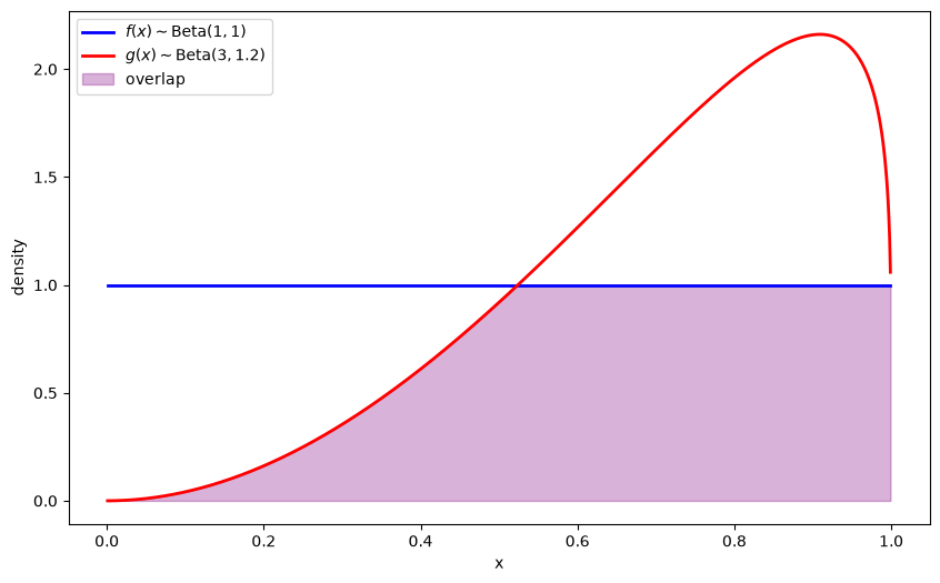
We introduce two Beta distributions \(f(x)\) and \(g(x)\), which we will use to illustrate the different divergence measures.
Let’s define parameters and density functions in Python
# Parameters in the two Beta distributions
F_a, F_b = 1, 1
G_a, G_b = 3, 1.2

@vectorize
def p(x, a, b):
    r = gamma(a + b) / (gamma(a) * gamma(b))
    return r * x** (a-1) * (1 - x) ** (b-1)

# The two density functions
f = jit(lambda x: p(x, F_a, F_b))
g = jit(lambda x: p(x, G_a, G_b))

# Plot the distributions
x_range = np.linspace(0.001, 0.999, 1000)
f_vals = [f(x) for x in x_range]
g_vals = [g(x) for x in x_range]

plt.figure(figsize=(10, 6))
plt.plot(x_range, f_vals, 'b-', linewidth=2, label=r'$f(x) \sim \text{Beta}(1,1)$')
plt.plot(x_range, g_vals, 'r-', linewidth=2, label=r'$g(x) \sim \text{Beta}(3,1.2)$')

# Fill overlap region
overlap = np.minimum(f_vals, g_vals)
plt.fill_between(x_range, 0, overlap, alpha=0.3, color='purple', label='overlap')

plt.xlabel('x')
plt.ylabel('density')
plt.legend()
plt.show()
21.4. Kullback–Leibler divergence#
Our first divergence function is the Kullback–Leibler (KL) divergence.
For probability densities (or pmfs) \(f\) and \(g\) it is defined by
We can interpret \(D_{KL}(f\|g)\) as the expected excess log loss (expected excess surprisal) incurred when we use \(g\) while the data are generated by \(f\).
\(D_{KL}(f\|g) = +\infty\) unless \(f\) is absolutely continuous with respect to \(g\) (\(f \ll g\)), that is, unless \(g(x) > 0\) wherever \(f(x) > 0\).
It has several important properties:
Non-negativity (Gibbs’ inequality): \(D_{KL}(f\|g) \ge 0\) with equality if and only if \(f=g\) almost everywhere.
Asymmetry: \(D_{KL}(f\|g) \neq D_{KL}(g\|f)\) in general (hence it is not a metric)
Information decomposition: \(D_{KL}(f\|g) = H(f,g) - H(f)\), where \(H(f,g)\) is the cross entropy and \(H(f)\) is the Shannon entropy of \(f\).
Chain rule: For joint distributions \(f(x, y)\) and \(g(x, y)\), \(D_{KL}(f(x,y)\|g(x,y)) = D_{KL}(f(x)\|g(x)) + E_{f}\left[D_{KL}(f(y|x)\|g(y|x))\right]\)
Data processing inequality: if a Markov kernel \(\kappa\) maps \(x\) into a coarser signal \(y\), and \(f\kappa\) and \(g\kappa\) denote the induced distributions of \(y\), then \(D_{KL}(f\kappa\|g\kappa) \le D_{KL}(f\|g)\).
The data processing inequality says that garbling data cannot make \(f\) and \(g\) easier to tell apart.
The section on the data processing inequality and coarse-graining in Blackwell’s Theorem on Comparing Experiments connects it to Blackwell’s ordering of experiments.
JS divergence and Chernoff entropy, defined below, also satisfy the data processing inequality.
KL divergence plays a central role in statistical inference, including model selection and hypothesis testing.
Likelihood Ratio Processes describes a link between KL divergence and the expected log likelihood ratio.
A Problem that Stumped Milton Friedman connects KL divergence to the expected stopping time of a sequential probability ratio test.
Incorrect Models uses two KL divergences to determine the limit of a Bayesian’s posterior probability when the data come from a mixture of \(f\) and \(g\) that the Bayesian’s model excludes.
Let’s compute the KL divergence between our example distributions \(f\) and \(g\).
A U-shaped Beta density diverges at \(0\) or \(1\).
We integrate over all of \((0,1)\) and split the interval at \(1/2\) so that quad handles one endpoint singularity at a time.
def integrate(F):
    """Integrate F over (0, 1), splitting the interval at 1/2."""
    left, _ = quad(F, 0, 0.5, limit=200)
    right, _ = quad(F, 0.5, 1, limit=200)
    return left + right

def compute_KL(f, g):
    """
    Compute KL divergence KL(f, g) via numerical integration
    """
    def integrand(w):
        fw = f(w)
        gw = g(w)
        return fw * np.log(fw / gw)
    return integrate(integrand)

# Compute KL divergences between our example distributions
kl_fg = compute_KL(f, g)
kl_gf = compute_KL(g, f)

print(f"KL(f, g) = {kl_fg:.4f}")
print(f"KL(g, f) = {kl_gf:.4f}")
KL(f, g) = 0.7592
KL(g, f) = 0.3436
The asymmetry of KL divergence has important practical implications.
\(D_{KL}(f\|g)\) heavily penalizes regions where \(f > 0\) but \(g\) is close to zero, because \(f\) puts weight on the large values of \(\log(f/g)\) there.
\(D_{KL}(f\|g)\) barely penalizes regions where \(g > 0\) but \(f\) is close to zero, because \(f\) puts almost no weight there.
\(D_{KL}(g\|f)\) reverses these roles.
In our example, \(g\) vanishes at \(x = 0\) while \(f = 1\) there, so \(D_{KL}(f\|g)\) exceeds \(D_{KL}(g\|f)\).
21.5. Jensen-Shannon divergence#
Sometimes we want a symmetric measure of divergence that captures the difference between two distributions without favoring one over the other.
This often arises in applications like clustering, where we want to compare distributions without assuming one is the true model.
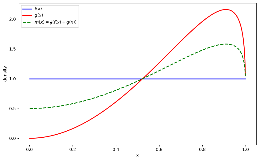
The Jensen-Shannon (JS) divergence symmetrizes KL divergence by comparing both distributions to their mixture:
where \(m\) is a mixture distribution that averages \(f\) and \(g\)
Let’s also visualize the mixture distribution \(m\):
def m(x):
    return 0.5 * (f(x) + g(x))

m_vals = [m(x) for x in x_range]

plt.figure(figsize=(10, 6))
plt.plot(x_range, f_vals, 'b-', linewidth=2, label=r'$f(x)$')
plt.plot(x_range, g_vals, 'r-', linewidth=2, label=r'$g(x)$')
plt.plot(x_range, m_vals, 'g--', linewidth=2, label=r'$m(x) = \frac{1}{2}(f(x) + g(x))$')

plt.xlabel('x')
plt.ylabel('density')
plt.legend()
plt.show()
The JS divergence has several useful properties:
Symmetry: \(JS(f,g)=JS(g,f)\).
Boundedness: \(0 \le JS(f,g) \le \log 2\).
Its square root \(\sqrt{JS}\) is a metric (Jensen–Shannon distance) on the space of probability distributions.
JS divergence equals the mutual information between a binary random variable \(Z \sim \text{Bernoulli}(1/2)\) indicating the source and a sample \(X\) drawn from \(f\) if \(Z=0\) or from \(g\) if \(Z=1\).
The Jensen–Shannon divergence appears in the original formulation of generative adversarial networks: when the discriminator is optimal, the generator minimizes \(2\, JS(p_{\text{data}}, p_{\text{model}}) - \log 4\) [Goodfellow et al., 2014].
Boundedness has a cost.
When two distributions have nearly disjoint supports, \(JS\) sits near its ceiling \(\log 2\) and is nearly flat in the parameters of the model, so gradient-based training stalls [Arjovsky and Bottou, 2017].
Let’s compute the JS divergence between our example distributions \(f\) and \(g\)
def compute_JS(f, g):
    """Compute Jensen-Shannon divergence."""
    def integrand(w):
        fw, gw = f(w), g(w)
        mw = 0.5 * (fw + gw)
        return 0.5 * fw * np.log(fw / mw) + 0.5 * gw * np.log(gw / mw)
    return integrate(integrand)

js_div = compute_JS(f, g)
print(f"Jensen-Shannon divergence JS(f,g) = {js_div:.4f}")
Jensen-Shannon divergence JS(f,g) = 0.0984
We can easily generalize to more than two distributions using the generalized Jensen-Shannon divergence with weights \(\alpha = (\alpha_i)_{i=1}^{n}\):
where:
\(\alpha_i \geq 0\) and \(\sum_{i=1}^n \alpha_i = 1\), and
\(H(f) = -\int f(x) \log f(x) dx\) is the differential entropy of density \(f\)
Unlike the entropy of a pmf, differential entropy can be negative: the uniform density on \([0, 1/2]\) has differential entropy \(-\log 2\).
\(JS_\alpha\) is nonnegative nonetheless, because \(H\) is concave.
21.6. Chernoff entropy#
Chernoff entropy originates from early applications of the theory of large deviations, which refines central limit approximations by providing exponential decay rates for rare events.
For densities \(f\) and \(g\) the Chernoff entropy, which Chernoff [1952] introduced and information theorists call the Chernoff information, is
Remarks:
The integral \(\rho(\phi)\) is the Chernoff coefficient.
At \(\phi=1/2\) it becomes the Bhattacharyya coefficient \(\int \sqrt{f g}\).
In binary hypothesis testing with \(T\) IID observations and equal prior probabilities on \(f\) and \(g\), the smallest attainable probability of error \(P_e(T)\) decays at exponential rate \(C(f,g)\): \(-\frac{1}{T} \log P_e(T) \rightarrow C(f,g)\).
Merging of Opinions: The Blackwell–Dubins Theorem calls the Bhattacharyya coefficient the Hellinger affinity.
Kakutani’s theorem there implies that when \(\int \sqrt{fg} < 1\), the distributions of infinite IID sequences drawn from \(f\) and from \(g\) are mutually singular.
We will see an example of the third point in the lecture Likelihood Ratio Processes, where we study the Chernoff entropy in the context of model selection.
Chernoff entropy lies between the Bhattacharyya distance \(-\log \int \sqrt{fg}\) and a combination of the two KL divergences:
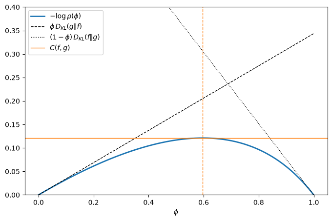
When \(f\) and \(g\) are positive on the same set, \(\log \rho(\phi)\) is a convex function of \(\phi\) that equals \(0\) at \(\phi = 0\) and \(\phi = 1\).
Its slope is \(-D_{KL}(g\|f)\) at \(\phi = 0\) and \(D_{KL}(f\|g)\) at \(\phi = 1\).
The lower bound in (21.5) evaluates \(\log \rho\) at \(\phi = 1/2\); the upper bound uses the two tangent lines at the endpoints, which lie below \(\log \rho\).
Exercise 21.2 asks you to prove these statements.
Let’s compute the Chernoff entropy between our example distributions \(f\) and \(g\) and check the bounds (21.5).
def chernoff_integrand(ϕ, f, g):
    """Integral entering Chernoff entropy for a given ϕ."""
    def integrand(w):
        return f(w)**ϕ * g(w)**(1-ϕ)
    return integrate(integrand)

def compute_chernoff_entropy(f, g):
    """Compute Chernoff entropy C(f,g)."""
    def objective(ϕ):
        return chernoff_integrand(ϕ, f, g)
    result = minimize_scalar(objective, bounds=(1e-5, 1-1e-5), method='bounded')
    min_value = result.fun
    ϕ_optimal = result.x
    chernoff_entropy = -np.log(min_value)
    return chernoff_entropy, ϕ_optimal

C_fg, ϕ_optimal = compute_chernoff_entropy(f, g)
print(f"Chernoff entropy C(f,g) = {C_fg:.4f}")
print(f"Optimal ϕ = {ϕ_optimal:.4f}")

bhattacharyya = -np.log(chernoff_integrand(0.5, f, g))
kl_bound = kl_fg * kl_gf / (kl_fg + kl_gf)
print(f"{bhattacharyya:.4f} ≤ {C_fg:.4f} ≤ {kl_bound:.4f} "
      f"≤ {min(kl_fg, kl_gf):.4f}")
Chernoff entropy C(f,g) = 0.1212
Optimal ϕ = 0.5969
0.1169 ≤ 0.1212 ≤ 0.2365 ≤ 0.3436
21.7. Comparing divergence measures#
We now compare these measures across several pairs of Beta distributions.
For Beta densities, the KL divergence and the Chernoff coefficient have closed forms.
Let \(B(a,b)\) be the Beta function and \(\psi = \Gamma'/\Gamma\) the digamma function.
Then
and
Exercise 21.1 asks you to derive these formulas.
JS divergence has no closed form, so we compute it by numerical integration over \((0,1)\).
The integration must cover the whole interval: Beta\((0.1, 0.2)\) puts a quarter of its probability mass outside \([10^{-5}, 1-10^{-5}]\).
def KL_beta(a1, b1, a2, b2):
    """KL(Beta(a1, b1) ‖ Beta(a2, b2)) in closed form."""
    return (betaln(a2, b2) - betaln(a1, b1)
            + (a1 - a2) * digamma(a1) + (b1 - b2) * digamma(b1)
            + (a2 - a1 + b2 - b1) * digamma(a1 + b1))

def log_chernoff_coef_beta(ϕ, a1, b1, a2, b2):
    """log ρ(ϕ) for Beta(a1, b1) and Beta(a2, b2) in closed form."""
    return (betaln(ϕ * a1 + (1 - ϕ) * a2, ϕ * b1 + (1 - ϕ) * b2)
            - ϕ * betaln(a1, b1) - (1 - ϕ) * betaln(a2, b2))

def chernoff_beta(a1, b1, a2, b2):
    """Chernoff entropy and minimizing ϕ for two Beta densities."""
    res = minimize_scalar(log_chernoff_coef_beta, bounds=(0, 1),
                          args=(a1, b1, a2, b2), method='bounded')
    return -res.fun, res.x

mass_out = beta_dist.cdf(1e-5, 0.1, 0.2) + beta_dist.sf(1 - 1e-5, 0.1, 0.2)
print(f"Mass of Beta(0.1, 0.2) outside [1e-5, 1-1e-5] = {mass_out:.3f}")
Mass of Beta(0.1, 0.2) outside [1e-5, 1-1e-5] = 0.251
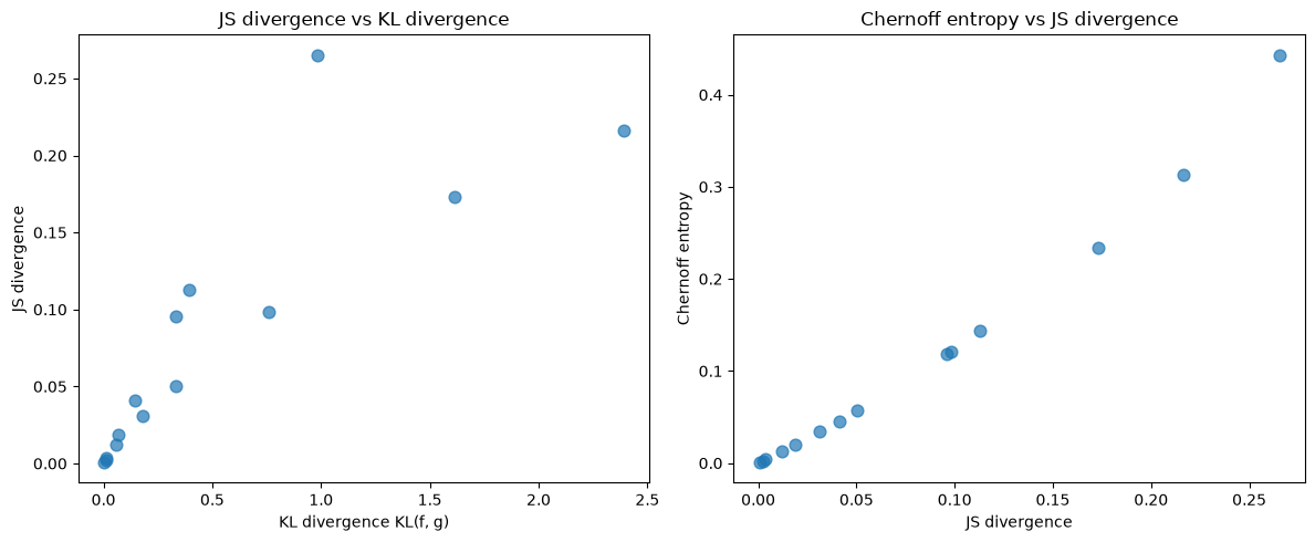
JS divergence and Chernoff entropy rank the fourteen pairs in the same order.
The two KL divergences rank them differently.
For \(g = \) Beta\((0.1, 0.2)\), \(KL(g, f)\) is by far the largest in the table, because \(g\) puts most of its mass near the endpoints, where \(g\) greatly exceeds \(f = 1\).
For \(g = \) Beta\((4, 1)\) and Beta\((5, 1)\), \(KL(f, g)\) exceeds its value for Beta\((0.1, 0.2)\), because these \(g\)’s vanish at \(0\), where \(f = 1\).
Next we visualize relationships among KL, JS, and Chernoff entropy.
kl_fg_values = [result['KL(f, g)'] for result in results]
js_values = [result['JS'] for result in results]
chernoff_values = [result['C'] for result in results]

fig, axes = plt.subplots(1, 2, figsize=(12, 5))

axes[0].scatter(kl_fg_values, js_values, alpha=0.7, s=60)
axes[0].set_xlabel('KL divergence KL(f, g)')
axes[0].set_ylabel('JS divergence')
axes[0].set_title('JS divergence vs KL divergence')

axes[1].scatter(js_values, chernoff_values, alpha=0.7, s=60)
axes[1].set_xlabel('JS divergence')
axes[1].set_ylabel('Chernoff entropy')
axes[1].set_title('Chernoff entropy vs JS divergence')

plt.tight_layout()
plt.show()
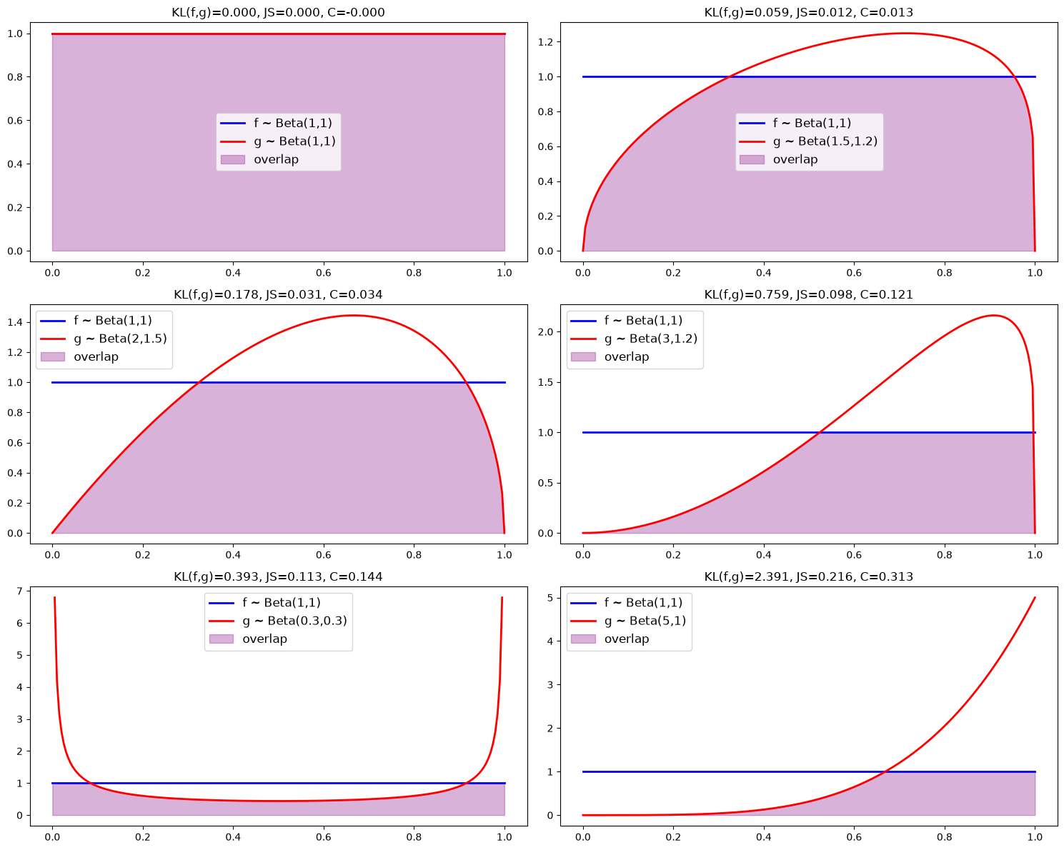
We now generate plots illustrating how overlap visually diminishes as divergence measures increase.
param_grid = [
    ((1, 1), (1, 1)),
    ((1, 1), (1.5, 1.2)),
    ((1, 1), (2, 1.5)),
    ((1, 1), (3, 1.2)),
    ((1, 1), (0.3, 0.3)),
    ((1, 1), (5, 1))
]
21.8. KL divergence and maximum-likelihood estimation#
Let \(x_1, x_2, \ldots, x_N\) be IID draws from a density \(p_0\).
A statistician fits a parametric family of densities \(\{p_\theta\}\) by maximum likelihood.
The empirical distribution \(p_e\) puts probability \(1/N\) on each observation:
where \(\delta(x - x_i)\) is the Dirac delta function centered at \(x_i\); it satisfies \(\delta(x - x_i) = 0\) for \(x \neq x_i\) and \(\int \delta(x - x_i) \, dx = 1\).
The log-likelihood function for parameter \(\theta\) is
The average log likelihood is an expectation under \(p_e\):
where \(H(p_e, p_\theta)\) is the cross-entropy defined in the primer above.
Maximum likelihood chooses \(\theta\) to minimize the cross-entropy \(H(p_e, p_\theta)\).
The KL divergence \(D_{KL}(p_e \| p_\theta)\) is of no use here.
When \(p_\theta\) is a density, \(p_e\) puts probability one on the finite set \(\{x_1, \ldots, x_N\}\), to which \(p_\theta\) assigns probability zero.
So \(p_e\) is not absolutely continuous with respect to \(p_\theta\), and \(D_{KL}(p_e \| p_\theta) = +\infty\) for every \(\theta\).
KL divergence enters through the population.
By the strong law of large numbers, for each \(\theta\)
where the equality is (21.3) for densities, and we assume that the entropy \(H(p_0)\) is finite.
The entropy \(H(p_0)\) does not depend on \(\theta\).
Maximum likelihood is the sample analogue of minimizing \(D_{KL}(p_0 \| p_\theta)\) over \(\theta\).
If \(p_0 = p_{\theta_0}\) for some \(\theta_0\), Gibbs’ inequality implies that \(\theta_0\) minimizes \(D_{KL}(p_0 \| p_\theta)\).
If no member of the family equals \(p_0\), then under regularity conditions the maximum likelihood estimator converges to the pseudo-true value
the member of the family closest to \(p_0\) in KL divergence [White, 1982].
Differentiating under the integral sign gives
The expected score is the negative gradient of the KL divergence, and it vanishes at \(\theta^*\).
Which Moments to Match? builds an estimator on this fact.
Maximum Likelihood Estimation describes how to compute maximum likelihood estimates.
Exercise 21.3 fits a misspecified Beta model to data drawn from a mixture.
21.10. Exercises#
Exercise 21.1
Let \(X \sim \text{Beta}(a, b)\), with density \(x^{a-1}(1-x)^{b-1}/B(a,b)\) on \((0,1)\).
Differentiate \(B(a,b) = \int_0^1 x^{a-1}(1-x)^{b-1} dx\) with respect to \(a\) and \(b\) to show that \(E \log X = \psi(a) - \psi(a+b)\) and \(E \log(1-X) = \psi(b) - \psi(a+b)\).
Use part 1 to derive the closed form for \(D_{KL}\bigl(\text{Beta}(a_1,b_1)\,\|\,\text{Beta}(a_2,b_2)\bigr)\) stated above.
Show that when \(f\) and \(g\) are Beta densities, \(f^\phi g^{1-\phi}\) is proportional to a Beta density, and use this fact to derive the closed form for \(\rho(\phi)\).
Let \(f = \text{Beta}(1,1)\) and \(g = \text{Beta}(0.1, 0.2)\). Compute \(KL(g, f)\), \(JS(f, g)\), and \(C(f, g)\) by applying
quadto the truncated interval \([10^{-5}, 1-10^{-5}]\). Compare the results with the values in the table above and explain the differences.
Solution
Part 1. Differentiating under the integral sign gives
Since \(B(a,b) = \Gamma(a)\Gamma(b)/\Gamma(a+b)\),
The same argument with \(b\) in place of \(a\) gives \(E \log(1-X) = \psi(b) - \psi(a+b)\).
Part 2. Let \(f = \text{Beta}(a_1, b_1)\) and \(g = \text{Beta}(a_2, b_2)\).
Then
Taking expectations under \(f\) and using part 1 gives
which rearranges to the formula in the text.
Part 3. Let \(a_\phi = \phi a_1 + (1-\phi) a_2\) and \(b_\phi = \phi b_1 + (1-\phi) b_2\).
Then
which is proportional to the Beta\((a_\phi, b_\phi)\) density.
Integrating over \((0,1)\) gives
Part 4. Here is code that repeats the computations on the truncated interval.
def KL_truncated(f, g):
    """KL(f, g) by quad over [1e-5, 1-1e-5]."""
    integrand = lambda w: f(w) * np.log(f(w) / g(w))
    return quad(integrand, 1e-5, 1 - 1e-5)[0]

def chernoff_truncated(f, g):
    """Chernoff entropy by quad over [1e-5, 1-1e-5]."""
    ρ = lambda ϕ: quad(lambda w: f(w)**ϕ * g(w)**(1-ϕ),
                       1e-5, 1 - 1e-5)[0]
    res = minimize_scalar(ρ, bounds=(0, 1), method='bounded')
    return -np.log(res.fun)

f_ex = jit(lambda x: p(x, 1, 1))
g_ex = jit(lambda x: p(x, 0.1, 0.2))
m_ex = lambda x: 0.5 * (f_ex(x) + g_ex(x))

truncated = [KL_truncated(g_ex, f_ex),
             0.5 * KL_truncated(f_ex, m_ex) + 0.5 * KL_truncated(g_ex, m_ex),
             chernoff_truncated(f_ex, g_ex)]
accurate = [KL_beta(0.1, 0.2, 1, 1),
            compute_JS(f_ex, g_ex),
            chernoff_beta(1, 1, 0.1, 0.2)[0]]

for name, t, a in zip(['KL(g, f)', 'JS(f, g)', 'C(f, g)'], truncated, accurate):
    print(f"{name}: truncated = {t:.4f}, accurate = {a:.4f}")
print(f"Mass of g outside the truncated interval = {mass_out:.4f}")
KL(g, f): truncated = 1.0036, accurate = 4.9773
JS(f, g): truncated = 0.1783, accurate = 0.2652
C(f, g): truncated = 0.4556, accurate = 0.4431
Mass of g outside the truncated interval = 0.2509
The density \(g = \text{Beta}(0.1, 0.2)\) puts a quarter of its mass outside \([10^{-5}, 1-10^{-5}]\), where \(g\) is enormous and \(f = 1\).
The omitted part of \(KL(g, f) = \int g \log g\) is large, because \(\log g\) is large there.
The omitted part of \(JS(f, g)\) is close to \(\frac{1}{2} \times 0.25 \times \log 2 \approx 0.087\), because \(g \log\bigl(2g/(f+g)\bigr) \approx g \log 2\) where \(g \gg f\).
Truncation also omits part of \(\rho(\phi)\), which lowers \(\rho\) and raises the computed Chernoff entropy.
Exercise 21.2
Let \(f\) and \(g\) be densities that are positive on the same set, and let \(\rho(\phi) = \int f^\phi g^{1-\phi} dx\).
Use Hölder’s inequality to show that \(\log \rho(\phi)\) is convex on \([0,1]\).
Show that \(\log\rho(0) = \log\rho(1) = 0\), that the derivative of \(\log \rho\) at \(\phi = 0\) is \(-D_{KL}(g\|f)\), and that its derivative at \(\phi = 1\) is \(D_{KL}(f\|g)\).
Deduce the bounds (21.5).
Verify the bounds numerically for every pair in the table above, and plot \(-\log\rho(\phi)\) together with the two tangent lines for our example \(f\) and \(g\).
Solution
Part 1. Take \(\phi_1, \phi_2 \in [0,1]\), \(\lambda \in (0,1)\), and \(\phi = \lambda \phi_1 + (1-\lambda) \phi_2\).
Write
Hölder’s inequality with exponents \(1/\lambda\) and \(1/(1-\lambda)\) gives
Taking logarithms gives \(\log \rho(\phi) \le \lambda \log\rho(\phi_1) + (1-\lambda) \log\rho(\phi_2)\).
Part 2. Because \(f\) and \(g\) are positive on the same set, \(\rho(0) = \int g = 1\) and \(\rho(1) = \int f = 1\).
Differentiating under the integral sign gives
At \(\phi = 0\) the derivative is \(\int g \log(f/g) = -D_{KL}(g\|f)\).
At \(\phi = 1\) the derivative is \(\int f \log(f/g) = D_{KL}(f\|g)\).
Part 3. The lower bound holds because \(C(f,g) = -\min_\phi \log\rho(\phi) \ge -\log \rho(1/2)\).
A convex function lies above its tangent lines, so
Hence
The right side is largest where the two lines cross, at \(\phi = D_{KL}(f\|g)/\bigl(D_{KL}(f\|g) + D_{KL}(g\|f)\bigr)\), where it equals \(D_{KL}(f\|g)\, D_{KL}(g\|f)/\bigl(D_{KL}(f\|g) + D_{KL}(g\|f)\bigr)\).
Maximizing the left side over \(\phi\) gives the middle inequality.
The last inequality holds because \(xy/(x+y) \le \min\{x, y\}\) for positive \(x\) and \(y\).
Part 4. We check the bounds for every pair in the table.
for (f_a, f_b), (g_a, g_b) in distribution_pairs:
    K_fg = KL_beta(f_a, f_b, g_a, g_b)
    K_gf = KL_beta(g_a, g_b, f_a, f_b)
    lower = -log_chernoff_coef_beta(0.5, f_a, f_b, g_a, g_b)
    C, _ = chernoff_beta(f_a, f_b, g_a, g_b)
    upper = K_fg * K_gf / (K_fg + K_gf)
    holds = lower <= C <= upper <= min(K_fg, K_gf)
    print(f"Beta({g_a},{g_b}): {lower:.4f} ≤ {C:.4f} ≤ {upper:.4f} "
          f"≤ {min(K_fg, K_gf):.4f}  {holds}")
Beta(0.1,0.2): 0.3929 ≤ 0.4431 ≤ 0.8195 ≤ 0.9810  True
Beta(0.3,0.3): 0.1374 ≤ 0.1437 ≤ 0.2785 ≤ 0.3934  True
Beta(0.3,0.4): 0.1141 ≤ 0.1189 ≤ 0.2319 ≤ 0.3316  True
Beta(0.5,0.5): 0.0450 ≤ 0.0457 ≤ 0.0905 ≤ 0.1447  True
Beta(0.7,0.6): 0.0198 ≤ 0.0199 ≤ 0.0396 ≤ 0.0673  True
Beta(0.9,0.8): 0.0039 ≤ 0.0039 ≤ 0.0077 ≤ 0.0142  True
Beta(1.1,1.05): 0.0007 ≤ 0.0007 ≤ 0.0014 ≤ 0.0026  True
Beta(1.2,1.1): 0.0025 ≤ 0.0025 ≤ 0.0049 ≤ 0.0092  True
Beta(1.5,1.2): 0.0125 ≤ 0.0126 ≤ 0.0251 ≤ 0.0437  True
Beta(2,1.5): 0.0334 ≤ 0.0339 ≤ 0.0673 ≤ 0.1081  True
Beta(2.5,1.8): 0.0562 ≤ 0.0577 ≤ 0.1138 ≤ 0.1731  True
Beta(3,1.2): 0.1169 ≤ 0.1212 ≤ 0.2365 ≤ 0.3436  True
Beta(4,1): 0.2231 ≤ 0.2341 ≤ 0.4564 ≤ 0.6363  True
Beta(5,1): 0.2939 ≤ 0.3128 ≤ 0.6047 ≤ 0.8094  True
The next figure plots \(-\log \rho(\phi)\) and the two tangent lines for \(f = \text{Beta}(1,1)\) and \(g = \text{Beta}(3,1.2)\).
ϕ_grid = np.linspace(0, 1, 200)
K_fg = KL_beta(F_a, F_b, G_a, G_b)
K_gf = KL_beta(G_a, G_b, F_a, F_b)
C_ex, ϕ_star = chernoff_beta(F_a, F_b, G_a, G_b)

fig, ax = plt.subplots(figsize=(8, 5))
ax.plot(ϕ_grid, -log_chernoff_coef_beta(ϕ_grid, F_a, F_b, G_a, G_b),
        lw=2, label=r'$-\log \rho(\phi)$')
ax.plot(ϕ_grid, ϕ_grid * K_gf, 'k--', lw=1,
        label=r'$\phi \, D_{KL}(g\|f)$')
ax.plot(ϕ_grid, (1 - ϕ_grid) * K_fg, 'k:', lw=1,
        label=r'$(1-\phi) \, D_{KL}(f\|g)$')
ax.axhline(C_ex, color='C1', lw=1, label=r'$C(f,g)$')
ax.axvline(ϕ_star, color='C1', lw=1, ls='--')
ax.set_ylim(0, 0.4)
ax.set_xlabel(r'$\phi$')
ax.legend()
plt.show()
Exercise 21.3
Let the data \(x_1, \ldots, x_N\) be IID draws from the mixture
of our example densities \(f = \text{Beta}(1,1)\) and \(g = \text{Beta}(3, 1.2)\).
A statistician fits the Beta\((a, b)\) family by maximum likelihood.
The family excludes \(h\).
Show that the pseudo-true value \((a^*, b^*) = \arg\min_{a,b} D_{KL}\bigl(h \,\|\, \text{Beta}(a,b)\bigr)\) solves \(\psi(a) - \psi(a+b) = E_h \log X\) and \(\psi(b) - \psi(a+b) = E_h \log (1-X)\).
Show that the maximum likelihood estimator \((\hat a_N, \hat b_N)\) solves the same equations with the expectations replaced by the sample means of \(\log x_i\) and \(\log(1-x_i)\).
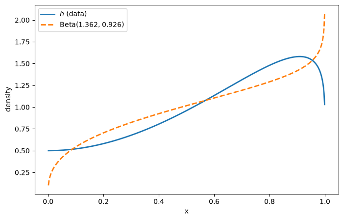
Compute \((a^*, b^*)\) and plot \(h\) against the Beta\((a^*, b^*)\) density.
Simulate samples of size \(N = 10^2, 10^3, \ldots, 10^6\) and verify that \((\hat a_N, \hat b_N)\) approaches \((a^*, b^*)\).
Solution
Parts 1 and 2. The log density of Beta\((a,b)\) is
Hence
with \(s_1 = E_h \log X\) and \(s_2 = E_h \log(1-X)\).
The average negative log likelihood is \(-\ell_N(a,b)/N = Q(a, b; \hat s_1, \hat s_2)\), where \(\hat s_1\) and \(\hat s_2\) are the sample means of \(\log x_i\) and \(\log(1-x_i)\).
The function \(\log B(a,b)\) is convex, so \(Q\) is convex in \((a, b)\).
By part 1 of Exercise 21.1, \(\partial \log B(a,b)/\partial a = \psi(a) - \psi(a+b)\) and \(\partial \log B(a,b)/\partial b = \psi(b) - \psi(a+b)\).
Setting the gradient of \(Q\) to zero gives the stated equations, with \((s_1, s_2)\) for the pseudo-true value and \((\hat s_1, \hat s_2)\) for the maximum likelihood estimator.
Part 3. Part 1 of Exercise 21.1 and linearity of expectations give \(s_1\) and \(s_2\) in closed form.
We minimize \(Q\) over \((\log a, \log b)\) to keep \(a\) and \(b\) positive.
from scipy.optimize import minimize

def Q(z, s1, s2):
    a, b = np.exp(z)
    return betaln(a, b) - (a - 1) * s1 - (b - 1) * s2

def fit_beta(s1, s2):
    res = minimize(Q, x0=np.zeros(2), args=(s1, s2), method='BFGS')
    return np.exp(res.x)

E_log_x = lambda a, b: digamma(a) - digamma(a + b)
s1 = 0.5 * E_log_x(F_a, F_b) + 0.5 * E_log_x(G_a, G_b)
s2 = 0.5 * E_log_x(F_b, F_a) + 0.5 * E_log_x(G_b, G_a)

a_star, b_star = fit_beta(s1, s2)
print(f"pseudo-true value: a* = {a_star:.4f}, b* = {b_star:.4f}")

h = lambda x: 0.5 * p(x, F_a, F_b) + 0.5 * p(x, G_a, G_b)
p_star = lambda x: p(x, a_star, b_star)
print(f"KL(h, Beta(a*, b*)) = {compute_KL(h, p_star):.4f}")

x_grid = np.linspace(0.001, 0.999, 500)
plt.figure(figsize=(8, 5))
plt.plot(x_grid, h(x_grid), lw=2, label='$h$ (data)')
plt.plot(x_grid, p_star(x_grid), lw=2, ls='--',
         label=f'Beta({a_star:.3f}, {b_star:.3f})')
plt.xlabel('x')
plt.ylabel('density')
plt.legend()
plt.show()
pseudo-true value: a* = 1.3621, b* = 0.9255
KL(h, Beta(a*, b*)) = 0.0124
Part 4. We draw samples from \(h\) and compute \((\hat a_N, \hat b_N)\) from the sample moments.
rng = np.random.default_rng(1234)

for N in [10**2, 10**3, 10**4, 10**5, 10**6]:
    from_f = rng.random(N) < 0.5
    x = np.where(from_f, rng.beta(F_a, F_b, N), rng.beta(G_a, G_b, N))
    a_hat, b_hat = fit_beta(np.mean(np.log(x)), np.mean(np.log1p(-x)))
    print(f"N = {N:>7}: a_hat = {a_hat:.4f}, b_hat = {b_hat:.4f}")
N =     100: a_hat = 1.2524, b_hat = 0.9221
N =    1000: a_hat = 1.5154, b_hat = 0.9324
N =   10000: a_hat = 1.3437, b_hat = 0.9186
N =  100000: a_hat = 1.3472, b_hat = 0.9216
N = 1000000: a_hat = 1.3601, b_hat = 0.9258
The estimates approach \((a^*, b^*)\), the member of the Beta family closest to \(h\) in KL divergence.
Incorrect Models studies a Bayesian whose model contains only \(f\) and \(g\) and who sees data from \(h\); KL divergences from \(h\) to \(f\) and to \(g\) determine where that Bayesian’s beliefs settle.
Which Moments to Match? uses the pseudo-true value of an auxiliary model as the target of an estimator.